| Table 1 | |
| Weights for MPRTE (Carneiro, Heckman and Vytlacil 2010) | |
| policy | weight_formula |
|---|---|
| Z + alpha (shift one instrument) | \(h(x, u_S) = f_{V|X}(u_S) / f_{P|X}(u_S)\) |
| P + alpha (uniform shift in P) | \(h(x, u_S) = f_{P|X}(u_S)\) |
| (1 + alpha) P (proportional shift) | \(h(x, u_S) = u_S f_{P|X}(u_S)\) |
Replication with R
Estimating Marginal Returns to Education (Carneiro, Heckman and Vytlacil 2011)
Introduction
R replication of tables in (Carneiro, Heckman, and Vytlacil 2011) following the AER replication package in replication_aer/. For the narrative walkthrough (research questions, identification, reproducibility), start with the replication guide. For commands and env vars, see the minimum runnable checklist.
Shared modules:
chv2011-data-prep.R— data merge, propensity score, bootstrap samplesgetboot.R— R port of Statagetboot.do(replication_aer/bootdata/)chv2011-table4a-core.R+export_data_with_tuition.R— Table 4(a) input and testchv2011-mte-core.R— semiparametric MTE and treatment parameterschv2011-gt-quarto.R—gttable helpers
Data mode: bundled_aligned — Merging basicvariables.dta and localvariables.dta by row order (author-aligned replication bundle; N should be 1747).
P0 merge: Bundled files use row-order alignment (bundled_aligned). Core Table A-3 statistics match; local instruments are approximate until geocode merge (P1 dataset.dta).
P1 bootstrap: Run Rscript 04-topics/rep-chv2011/Rcode/getboot.R to create replication_aer/bootdata/.
P2 Table 4(a): Run export_data_with_tuition.R then Table_4a.R with CHV2011_BOOT_4A=1000 for author-matching bootstrap p-values.
P3 MTE / treatment parameters: Run Table_4b.R, Table_5.R, and run_all_figures.R with CHV2011_BOOT=250 for bootstrap SEs. Semiparametric MTE uses the Table 4(a) polynomial proxy; normal-model Figure 1 / Table 5 col 1 use shipped normalmodel/mtexvb.out.
Set rerun_script <- TRUE in chunk rerun-table-scripts to re-estimate (slow; use env vars CHV2011_BOOT, CHV2011_BOOT_4A to control bootstrap replications).
Each table and figure below includes a replication note with: how to reproduce it, current completion status, and known limitations. Status labels:
| Label | Meaning |
|---|---|
| Complete | Display or estimation matches the paper closely on bundled data |
| Partial | Pipeline implemented and run at paper bootstrap \(B\); some numbers deviate from the published table |
| Display only | Static definitions / glossary — no econometric re-estimation |
| Author track | Requires Stata / GAUSS / MATLAB outputs not produced in the R course pipeline |
R scripts and cached results
Download scripts and .RData objects from Rcode/. Re-run a single table: Rscript 04-topics/rep-chv2011/Rcode/Table_3.R (see per-table notes for env vars).
Main text tables
Table 1
NoteReplication notes — Table 1
- Procedure: Static display of MPRTE policy weights from the paper (Table 1). Script:
Table_1.R— no data merge or estimation. - Status: Display only — formulas transcribed for reference.
- Caveats: None; this table documents notation used in Tables 5 and 6.
Table 2
| Table 2 | ||
| Definitions of variables used in the empirical analysis | ||
| symbol | definition | source |
|---|---|---|
| Y | Log average hourly wage 1989-1993 (1983 dollars) | Outcome |
| S | College attendance (ever attended vs HS grad only) | Treatment |
| X | AFQT, mother education, siblings, urban, local labor market, experience, cohort | Controls |
| \(Z \ X\) | College proximity at 14, local wage/unemployment/tuition at 17 (with X interactions) | IV |
NoteReplication notes — Table 2
- Procedure: Variable glossary (\(Y\), \(S\), \(X\), \(Z\)). Script:
Table_2.R. - Status: Display only.
- Caveats: Local instruments in \(Z \setminus X\) (
pub4,tuition,lwage5, …) are only approximate under the bundled row-merge (see Table A-3).
Table 3
| Table 3 | ||
| College decision model — average marginal derivatives | ||
| label | cell | |
|---|---|---|
| CONTROLS (X): | Corrected AFQT | 0.2866*** (0.0115) |
| Mother’s Years of Schooling | 0.0438*** (0.0063) | |
| Number of Siblings | -0.0268*** (0.0078) | |
| Urban Residence at 14 | 0.0660** (0.0290) | |
| “Permanent” Local Log Earnings at 17 | 0.1803* (0.0973) | |
| “Permanent” State Unemployment Rate at 17 | 0.0155 (0.0152) | |
| INSTRUMENTS (Z): | Presence of a College at 14 | 0.0185 (0.0267) |
| Local Log Earnings at 17 | -0.2021** (0.0985) | |
| Local Unemployment Rate at 17 (in %) | -0.0130 (0.0087) | |
| Tuition in 4 Year Public Colleges at 17 (in $100) | 0.0021 (0.0017) | |
| Test for joint significance of instruments: p-value | 0.8450 | |
NoteReplication notes — Table 3
- Procedure: (1) Merge data via
chv2011-data-prep.R. (2) Logit first step on full \(N = 1747\). (3) Average marginal derivatives withdnorm(xbeta)per authoravder_ddd.do. (4) Bootstrap SEs from cachedbootdata/(rungetboot.Rfirst). Command:CHV2011_BOOT=250 Rscript Rcode/Table_3.R. - Status: Partial — cached at \(B = 250\); control-variable derivatives align with the paper; bootstrap SEs displayed.
- Caveats: Instrument average derivatives and the joint LR test (\(p = 0.0001\) in the paper) require geocode-merged
dataset.dta(getdataset.do). Bundled merge gives joint IV \(p \approx 0.85\).
Table 4(a)
| Table 4(a) | |||
| Linearity of E(Y|X,P); Romano-Wolf critical value (10%) = 0.027; joint: Fail to reject | |||
| polynomial_order | Asymptotic p-value | cell | reject |
|---|---|---|---|
| 2 | 0.0222 | 0.1440 | Fail to reject |
| 3 | 0.0685 | 0.2500 | Fail to reject |
| 4 | 0.1110 | 0.4940 | Fail to reject |
| 5 | 0.0986 | 0.4590 | Fail to reject |
NoteReplication notes — Table 4(a)
- Procedure: (1) Export analysis data:
Rscript Rcode/export_data_with_tuition.R. (2) Port of authorbootstrap_MT.R: probit first step, OLS of \(Y\) on \(X\), \(P\), \(P^2,\ldots\), pivotal bootstrap Wald, Romano–Wolf 10% critical value. Command:CHV2011_BOOT_4A=1000 Rscript Rcode/Table_4a.R(~40 min). - Status: Partial — run complete at \(B = 1000\); Murphy–Topel and HC asymptotic \(p\)-values reported alongside bootstrap \(p\)-values.
- Caveats: On bundled data, HC asymptotic \(p\) for degree-2 polynomial \(\approx 0.035\) (matches paper); bootstrap \(p\)-values (0.14–0.49) and RW joint test fail to reject, unlike the paper. Author uses probit here but logit in the main choice equation.
Table 4(b)
| Table 4(b) | ||
| Test of equality of adjacent LATEs (joint p = 0.000; bootstrap bootdata, B = 250) | ||
| Interval 1 | Interval 2 | LATE diff |
|---|---|---|
| 0-0.04 | 0.04-0.08 | -0.1151 (0.1251) |
| 0.08-0.12 | 0.12-0.16 | -0.0875 (0.0849) |
| 0.16-0.2 | 0.2-0.24 | -0.0648 (0.0530) |
| 0.24-0.28 | 0.28-0.32 | -0.0470 (0.0303) |
| 0.32-0.36 | 0.36-0.4 | -0.0342* (0.0187) |
| 0.4-0.44 | 0.44-0.48 | -0.0263 (0.0171) |
| 0.48-0.52 | 0.52-0.56 | -0.0233 (0.0177) |
| 0.56-0.6 | 0.6-0.64 | -0.0252 (0.0186) |
| 0.64-0.68 | 0.68-0.72 | -0.0321 (0.0267) |
| 0.72-0.76 | 0.76-0.8 | -0.0439 (0.0457) |
| 0.8-0.84 | 0.84-0.88 | -0.0606 (0.0745) |
| 0.88-0.92 | 0.92-0.96 | -0.0822 (0.1120) |
NoteReplication notes — Table 4(b)
- Procedure: Polynomial MTE from the Table 4(a) outcome spec (
chv2011-mte-core.R); test equality of adjacent LATE bins on a \(u_S\) grid; bootstrap \(p\)-values frombootdata/. Command:CHV2011_BOOT=250 Rscript Rcode/Table_4b.R. - Status: Partial — cached at \(B = 250\); joint test rejects adjacent LATE equality (pattern similar to paper: declining MTE).
- Caveats: Author pipeline: GAUSS
superboot→mte1.out…mte250.out→ MATLABmte4c.m. R uses a polynomial proxy, not GAUSSchv01b.prg; LATE bin definitions and difference sign convention differ frommte4c.m.
Table 5
| Table 5 | ||
| Returns to a year of college (Normal vs semiparametric; annualized) | ||
| parameter | normal | semiparam |
|---|---|---|
| Average Treatment Effect (ATE) | 0.0660 (NA) |
Not Identified |
| Treatment on the Treated (TT) | 0.0300 (NA) |
Not Identified |
| Treatment on the Untreated (TUT) | 0.1020 (NA) |
Not Identified |
| MPRTE: Z + alpha | 0.0660 (NA) |
0.0378 (0.0758) |
| MPRTE: P + alpha | 0.0660 (NA) |
0.0478 (0.0974) |
| MPRTE: (1 + alpha) P | 0.0300 (NA) |
-0.1507 (0.1920) |
| Linear IV (P(Z)) | 0.1186 (NA) |
0.1186 (0.1173) |
| OLS | 0.0767 (NA) |
0.0767 (0.0070) |
NoteReplication notes — Table 5
- Procedure: Two columns. Normal: treatment parameters from shipped
normalmodel/mtexvb.out(authornormalselb.do). Semiparametric: MPRTE (three policy weights), linear IV, OLS viachv2011-mte-core.R; bootstrap SEs for semiparametric rows. Command:CHV2011_BOOT=250 Rscript Rcode/Table_5.R. - Status: Partial — cached at \(B = 250\). IV (\(\approx 0.12\)) and OLS (\(\approx 0.08\)) annual returns are close in magnitude to the paper; normal ATE \(\approx 0.066\) matches.
- Caveats: Semiparametric ATE/TT/TUT marked not identified without \(f(u_S \mid X)\) (needs GAUSS
cdens). Semiparametric MPRTE deviates from paper col. 2 (polynomial vschv01b.prg). Normal-column bootstrap SEs not replicated (authornormalsel_boot.do).
Table 6(a)
| Table 6(a) | |||
| Returns — sensitivity (outcome / sample); bootstrap B = 250 (R polynomial MTE core) | |||
| parameter | Baseline | No dropouts | Dropout dummies in wage eq. |
|---|---|---|---|
| ATE (tilde) | 0.0441 (0.0886) |
0.0910 (0.0935) |
0.0015 (0.0893) |
| TT (tilde) | 0.1571 (0.0945) |
0.2428 (0.1221) |
0.1218 (0.0940) |
| TUT (tilde) | -0.0787 (0.1304) |
-0.1112 (0.1235) |
-0.1215 (0.1275) |
| MPRTE (|Z gamma - V| < e) | 0.0378 (0.0758) |
0.0806 (0.0791) |
0.0059 (0.0767) |
Table 6(b)
| Table 6(b) | |||||
| Returns — sensitivity (choice equation); SLS column cached from paper; B = 250 | |||||
| parameter | All X in Z | No Z x X interactions | Cameron-Taber IVs | No tuition IV | SLS index (author cached) |
|---|---|---|---|---|---|
| ATE (tilde) | 0.0939 (0.0739) |
0.0102 (0.1115) |
-0.0108 (0.1707) |
0.0204 (0.1422) |
0.0871 |
| TT (tilde) | 0.1812 (0.0693) |
0.1526 (0.1528) |
0.0745 (0.2370) |
0.1771 (0.1980) |
0.2154 |
| TUT (tilde) | -0.0091 (0.0912) |
-0.1449 (0.1834) |
-0.1063 (0.2538) |
-0.1500 (0.2201) |
-0.0337 |
| MPRTE (|Z gamma - V| < e) | 0.0793 (0.0609) |
0.0006 (0.0965) |
-0.0205 (0.1482) |
0.0083 (0.1226) |
0.0799 |
NoteReplication notes — Table 6(a) & 6(b)
- Procedure: Eight robustness columns via
run_chv2011_spec()— baseline, no dropouts, dropout dummies (6a); all \(X\) in \(Z\), no \(Z \times X\), Cameron–Taber IV set, no tuition, SLS (6b). Each column re-estimates MTE + \(\tilde{\text{ATE}}\), \(\tilde{\text{TT}}\), \(\tilde{\text{TUT}}\), MPRTE\(_Z\). Command:CHV2011_BOOT=250 Rscript Rcode/Table_6.R(~7 min). - Status: Partial — cached at \(B = 250\) for all non-SLS columns. SLS column: Display only (author paper coefficients cached;
npindexnot run). - Caveats: R polynomial MTE core, not GAUSS
cdens+treatparnew.m. Baseline \(\tilde{\text{ATE}} = 0.044\) vs paper \(0.082\); no-dropouts TT closer (0.243 vs 0.261). Nodrop bootstrap SEs ideally needtable6/bootdata_nodrop/(authorgetboot.do).
Web Appendix Tables
Table A-1
| Table A-1 | ||
| Weight definitions (Heckman and Vytlacil 2005) | ||
| parameter | definition | weight |
|---|---|---|
| Table A-1A: Treatment effects as weighted averages of MTE | ||
| ATE | Integral of MTE against weight h_ATE(x, u_S) | |
| TT | Integral of MTE against weight h_TT(x, u_S) = 1{S=1} | |
| TUT | Integral of MTE against weight h_TUT(x, u_S) = 1{S=0} | |
| PRTE | Policy-relevant TE for a discrete policy change | |
| IV | Weighted average of MTE with instrument-specific weights | |
| OLS | Weighted average of MTE with OLS selection weights | |
| Table A-1B: Weights for ATE, TT, TUT, PRTE, IV and OLS | ||
| ATE | \(f_{P|X}(u_S)\) | |
| TT | \(1{P > u_S}\) | |
| TUT | \(1{P <= u_S}\) | |
| PRTE | Policy-specific (see Table 1) | |
| IV | \(f_{P|X}(u_S) * (Z - E[Z|X]) / E[Z|X,P=u_S]\) | |
| OLS | \(f_{P|X}(u_S) * (P - u_S)\) | |
NoteReplication notes — Table A-1
- Procedure: Static definitions of ATE, TT, TUT, PRTE, IV, and MPRTE policy weights. Script:
Table_A1.R. - Status: Display only.
- Caveats: None.
Table A-2
| Table A-2 | |
| Regression of AFQT on schooling (proxy; bundled corrected AFQT) | |
| term | cell |
|---|---|
| (Intercept) | -0.5738*** (0.0616) |
| hs_grad | 0.6509*** (0.0683) |
| some_college | 0.8744*** (0.0400) |
| state | NA (NA) |
NoteReplication notes — Table A-2
- Procedure: AFQT correction summary using bundled
cafqt(pre-corrected Hansen–Heckman–Mullen) and schooling-at-test proxies. Script:Table_A2.R. - Status: Partial — descriptive comparison on bundled data.
- Caveats: No author replication script in the AER package; bundled
cafqtis already corrected, so this table documents the adjustment rather than re-estimating it.
Table A-3
| Table A-3 | ||
| Sample statistics (S=0: N=882; S=1: N=865; merge: bundled_aligned) | ||
| variable | s0 | s1 |
|---|---|---|
| Log of Average Hourly Wage 1989-1993 | 2.2090 (0.4412) |
2.5497 (0.4959) |
| Years of Actual Experience | 10.1043 (3.1261) |
6.8404 (3.2523) |
| Corrected AFQT | -0.0447 (0.8674) |
0.9515 (0.7498) |
| Mother’s Years of Schooling | 11.3084 (2.1056) |
12.9121 (2.2790) |
| Number of Siblings | 3.2630 (2.0842) |
2.5850 (1.6450) |
| Urban Residence at 14 | 0.6995 (0.4587) |
0.7896 (0.4078) |
| Local Log Earnings in 1991 | 10.2921 (0.1630) |
10.2939 (0.1678) |
| Local Unemployment in 1991 (%) | 6.9071 (1.3348) |
6.7105 (1.1860) |
| Presence of a 4 Year College at 14 | 0.5091 (0.5002) |
0.5410 (0.4986) |
| Local Log Earnings at 17 | 10.2780 (0.1559) |
10.2736 (0.1710) |
| Local Unemployment Rate at 17 (%) | 7.1202 (1.8701) |
7.0442 (1.7556) |
| Tuition in 4 Year Public Colleges at 17 ($100) | 21.4162 (8.1444) |
21.7224 (7.8123) |
| Permanent Local Log Earnings at 17 | 10.2768 (0.1804) |
10.2895 (0.1950) |
| Permanent Local Unemployment Rate at 17 | 6.2801 (1.0063) |
6.2222 (0.9647) |
NoteReplication notes — Table A-3
- Procedure: Sample means by \(S\) from merged data; runs
validate_chv2011_merge()against paper targets. Script:Table_A3.R. Start here to verify P0 merge before other tables. - Status: Complete for core demographics (\(N = 1747\), 882/865, wage means match to rounding).
- Caveats: Local IV variables (
pub4,tuition,lwage5, …) deviate because bundled merge is row-order (cor(caseid, newid) \approx 0.88$), not geocodenewid.dta`.
Table A-4
| Table A-4 | ||
| College decision model — coefficients and average derivatives | ||
| label | coef_cell | deriv_cell |
|---|---|---|
| Corrected AFQT | -6.4256 (5.0189) |
0.2866*** (0.0118) |
| Mother’s Years of Schooling | -0.2733 (2.1463) |
0.0438*** (0.0066) |
| Number of Siblings | -0.4059 (2.4030) |
-0.0268*** (0.0083) |
| Urban Residence at 14 | 0.3386** (0.1401) |
0.0660** (0.0317) |
| “Permanent” Local Log Earnings at 17 | -54.1080* (29.1108) |
0.1803** (0.0825) |
| “Permanent” State Unemployment Rate at 17 | -0.0936 (0.6327) |
0.0155 (0.0152) |
| Presence of a College at 14 | 0.4641 (0.8731) |
0.0185 (0.0275) |
| Local Log Earnings at 17 | -1.5203 (2.7382) |
-0.2021** (0.0829) |
| Local Unemployment Rate at 17 (in %) | -0.1394 (0.2476) |
-0.0130 (0.0086) |
| Tuition in 4 Year Public Colleges at 17 (in $100) | 0.0114 (0.0595) |
0.0021 (0.0015) |
NoteReplication notes — Table A-4
- Procedure: Same logit + average-derivative pipeline as Table 3 on the men-only subsample. Command:
CHV2011_BOOT=250 Rscript Rcode/Table_A4.R. - Status: Partial — cached at \(B = 250\) (same P1
bootdata/resampling). - Caveats: Same IV / joint-test limitations as Table 3 on bundled data.
Table A-5
| Table A-5 | ||
| Linearity of E(Y|X,P) — double bootstrap for estimated P; RW critical (10%) = 0.0538; joint: Fail to reject | ||
| polynomial_order | cell | reject |
|---|---|---|
| 2 | 0.0940 | Fail to reject |
| 3 | 0.1780 | Fail to reject |
| 4 | 0.2800 | Fail to reject |
| 5 | 0.2780 | Fail to reject |
NoteReplication notes — Table A-5
- Procedure: Linearity test with double bootstrap for estimated \(P\) per
description1.tex/chv2011-table4a-core.R. Command:CHV2011_BOOT_A5_OUT=500 CHV2011_BOOT_A5_IN=100 Rscript Rcode/Table_A5.R(~5 h). - Status: Partial — run complete at 500×100; Romano–Wolf critical value \(\approx 0.054\) (paper \(\approx 0.052\)).
- Caveats: Bootstrap \(p\)-values (0.09–0.28) are much larger than the paper (0.004–0.026); joint test fails to reject where the paper rejects. Author
double_bootstrap.Ris not in the AER bundle; geocode merge may be required for numerical match.
Table A-6
| Table A-6 | |||
| Maximum likelihood estimates, normal switching regression (OLS-by-S proxy) | |||
| label | cell_mu1 | cell_mu0 | cell_diff |
|---|---|---|---|
| Experience | 0.0771 (0.0193) |
0.0607 (0.0215) |
0.0163 (0.0289) |
| Experience Squared | -0.0036 (0.0013) |
0.0002 (0.0012) |
-0.0038 (0.0017) |
| Corrected AFQT | 0.0645 (0.0323) |
0.0786 (0.0168) |
-0.0140 (0.0364) |
| Mother’s Years of Schooling | 0.0080 (0.0527) |
-0.0397 (0.0307) |
0.0477 (0.0610) |
| Number of Siblings | -0.0004 (0.0290) |
-0.0036 (0.0196) |
0.0032 (0.0350) |
| Urban Residence at 14 | 0.0852 (0.0410) |
0.0794 (0.0308) |
0.0057 (0.0513) |
| Permanent Local Log Earnings at 17 | 5.9795 (7.7007) |
-6.2991 (6.9519) |
12.2786 (10.3745) |
| Permanent State Unemployment at 17 | 0.1152 (0.1859) |
0.1644 (0.1390) |
-0.0492 (0.2321) |
| Local Log Earnings 1991 | -0.1083 (0.1185) |
0.1350 (0.1003) |
-0.2433 (0.1553) |
| Local Unemployment 1991 | 0.0004 (0.0180) |
-0.0106 (0.0141) |
0.0110 (0.0228) |
NoteReplication notes — Table A-6
- Procedure: Normal switching regression — separate OLS wage equations for \(S = 1\) and \(S = 0\) on trimmed sample. Script:
Table_A6.R. - Status: Partial — point estimates from R
lm(); no bootstrap SEs in this script. - Caveats: Author uses
normalmodel/normalselb.do+ bootstrap (normalsel_boot.do) for published SEs. Coefficient signs/magnitudes are informative but not paper-identical.
Table A-7
| Table A-7 | |
| Average derivatives, partially linear wage model (Robinson 1988) | |
| label | cell |
|---|---|
NoteReplication notes — Table A-7
- Procedure: Robinson (1988) partial linear model: \(Y = X'\beta_0 + g(P) + \varepsilon\); report average derivatives w.r.t. \(X\). Default
CHV2011_BOOT=50unless overridden. Script:Table_A7.R. - Status: Partial — R implementation complete; cached bootstrap may be below paper \(B = 250\).
- Caveats: Author uses GAUSS semi-parametric estimation; R uses a simpler partial-linear proxy. Re-run with
CHV2011_BOOT=250for tighter SEs.
Table A-8
| Table A-8 | |
| OLS and IV estimates of return to a year of college | |
| method | cell |
|---|---|
| OLS | -15.2282 (11.4800) |
| IV (P(Z)) | -15.6087 (17.0834) |
| IV (distance to college) | -0.8958 (3.6167) |
| IV (local wage at 17) | 0.1486 (0.2073) |
| IV (local unemployment at 17) | -1.1737 (1.1172) |
| IV (tuition at 17) | 0.1172 (3.1626) |
| 2SLS (all IVs) | 0.1186 (0.1111) |
NoteReplication notes — Table A-8
- Procedure: Linear IV and OLS returns to schooling; bootstrap SEs via
chv2011-mte-core.Restimate_ols_iv_returns(). DefaultCHV2011_BOOT=50. Script:Table_A8.R. - Status: Partial — R pipeline functional; cached bootstrap may be below paper \(B = 250\).
- Caveats: Author
./runboot0+getolsiv.doproducesolsiv*.out. IV relevance weaker on bundled merge.
Figures
All figures: Rscript 04-topics/rep-chv2011/Rcode/Figure_N.R or batch Rscript Rcode/run_all_figures.R. Outputs cached in Rcode/Figure_*.RData.
Figure 1
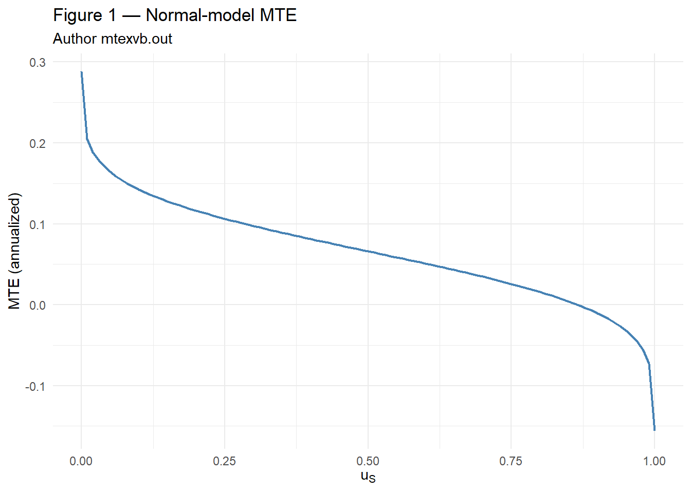
NoteReplication notes — Figure 1
- Procedure: Plot MTE curve from shipped
normalmodel/mtexvb.outviachv2011_fig_normal_mte(). Author:normalmodel/normalselb.do+ MATLABdofig1.m. - Status: Partial — uses author normal-model output file bundled with the replication package.
- Caveats: Curve shape follows author ML normal selection model; not re-estimated in R.
Figure 2
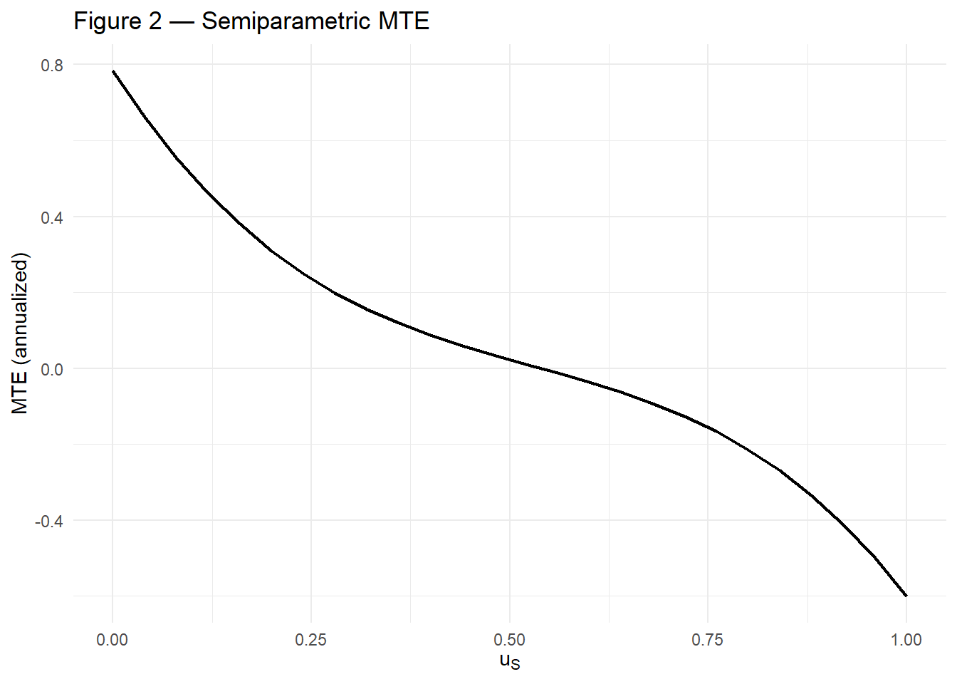
NoteReplication notes — Figure 2
- Procedure: Semiparametric MTE from polynomial outcome spec (
chv2011-mte-core.R). Author: GAUSSchv01b.prgonsuperbootoutput. - Status: Partial — qualitative declining MTE pattern; levels differ from published figure.
- Caveats: Author track for exact match requires
mainresults/out/mte*.outfrom./superboot.
Figure 3
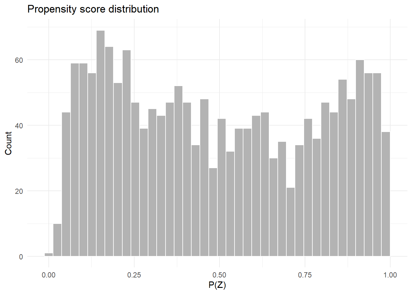
NoteReplication notes — Figure 3
- Procedure: Histogram / density of estimated \(P(X,Z)\) from logit first step (
chv2011_fig_phats()). - Status: Partial — distribution shape reasonable on bundled data.
- Caveats: Trimmed vs full sample may differ from author figure; local IV merge affects tail behavior.
Figure 4
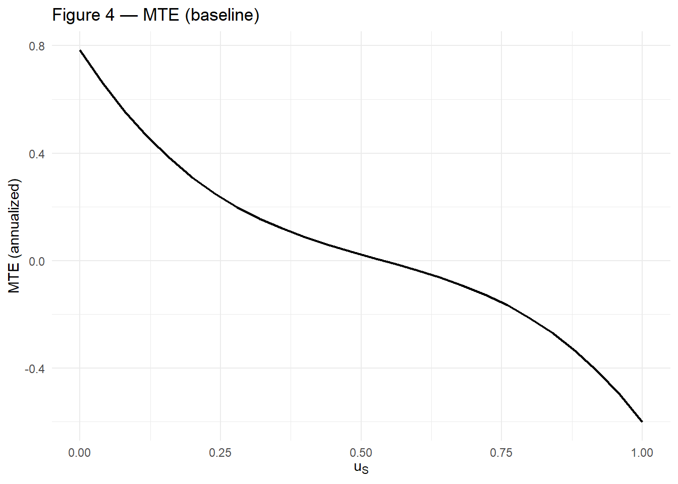
NoteReplication notes — Figure 4
- Procedure: Same polynomial MTE plot as Figure 2 with alternate title/layout (
chv2011_fig_mte()). - Status: Partial — same limitations as Figure 2.
- Caveats: Author Figure 4 may use a different trimming or binning rule in MATLAB.
Figure 5
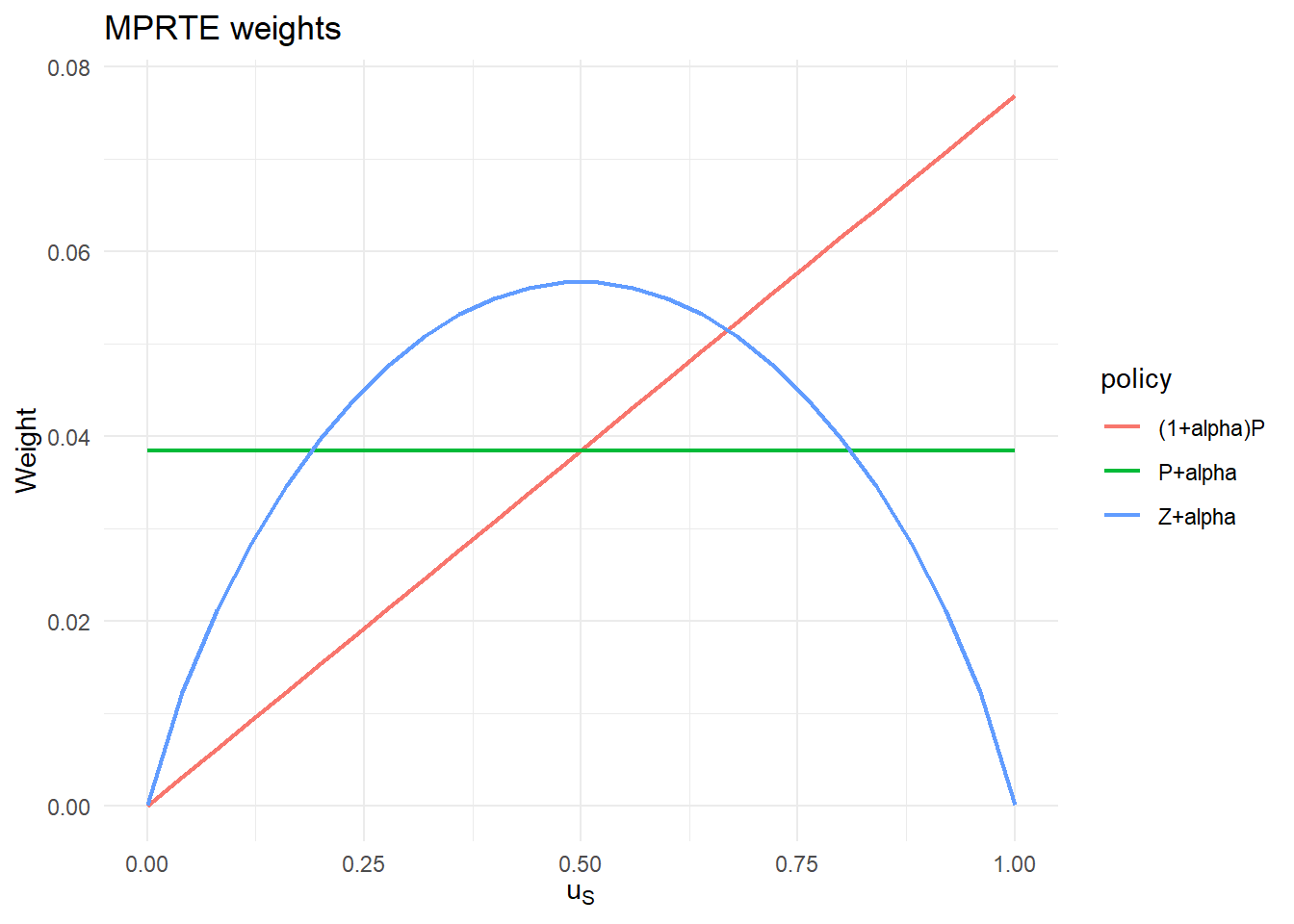
NoteReplication notes — Figure 5
- Procedure: Plot MPRTE integration weights \(h(x, u_S)\) over \(u_S\) (
chv2011_fig_weights()). - Status: Partial — illustrates three policy-weight schemes from Table 1.
- Caveats: Weights use R polynomial MTE and empirical \(f(P \mid X)\), not GAUSS density estimates.
Figure 6
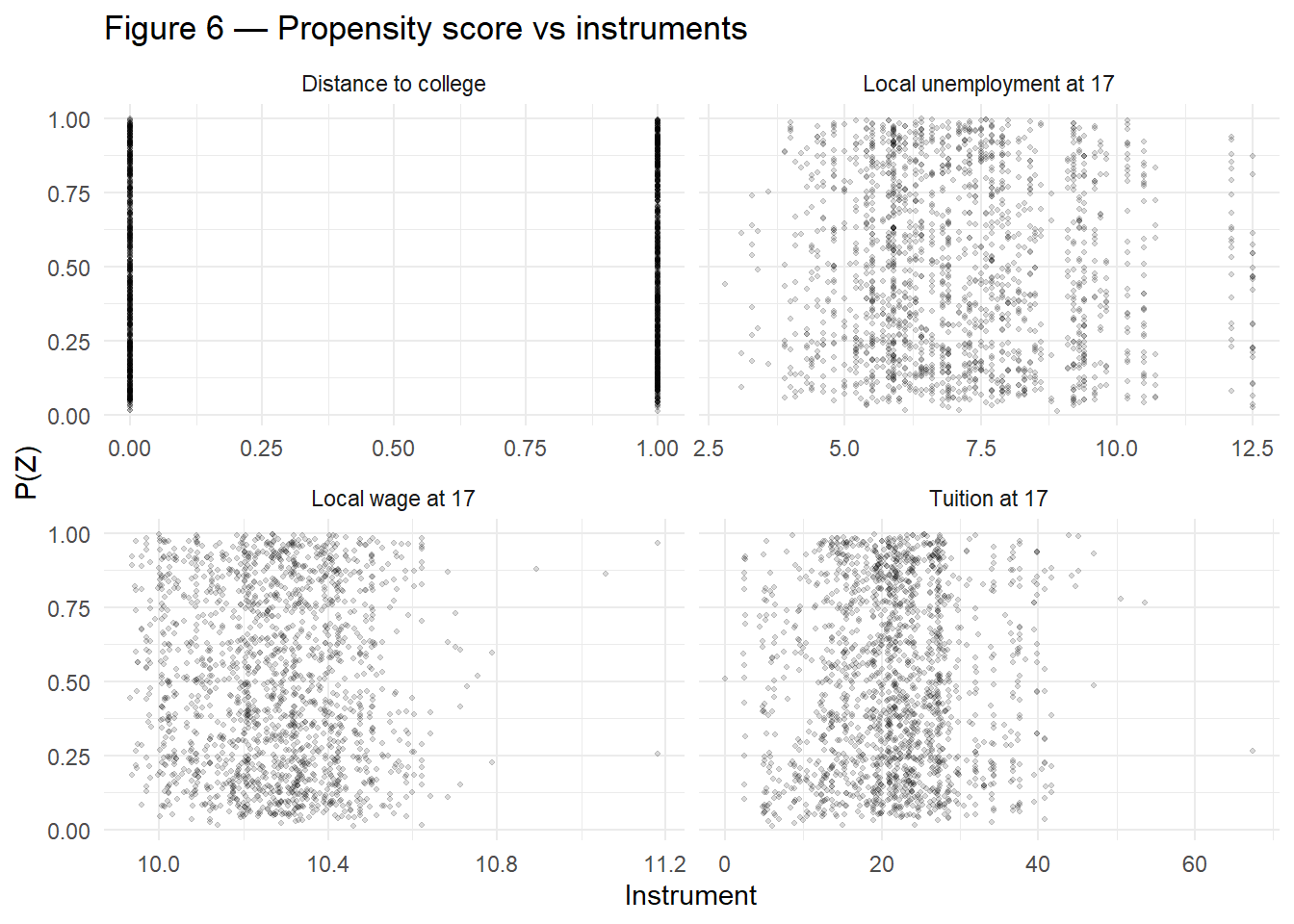
NoteReplication notes — Figure 6
- Procedure: Scatter of propensity vs excluded instruments (
chv2011_fig_iv_support()) to visualize IV relevance. - Status: Partial — useful diagnostic on bundled data.
- Caveats: Instrument–\(P\) relationships differ from the paper under row-merge; geocode
dataset.dtaneeded for exact support plot.
Figure 7
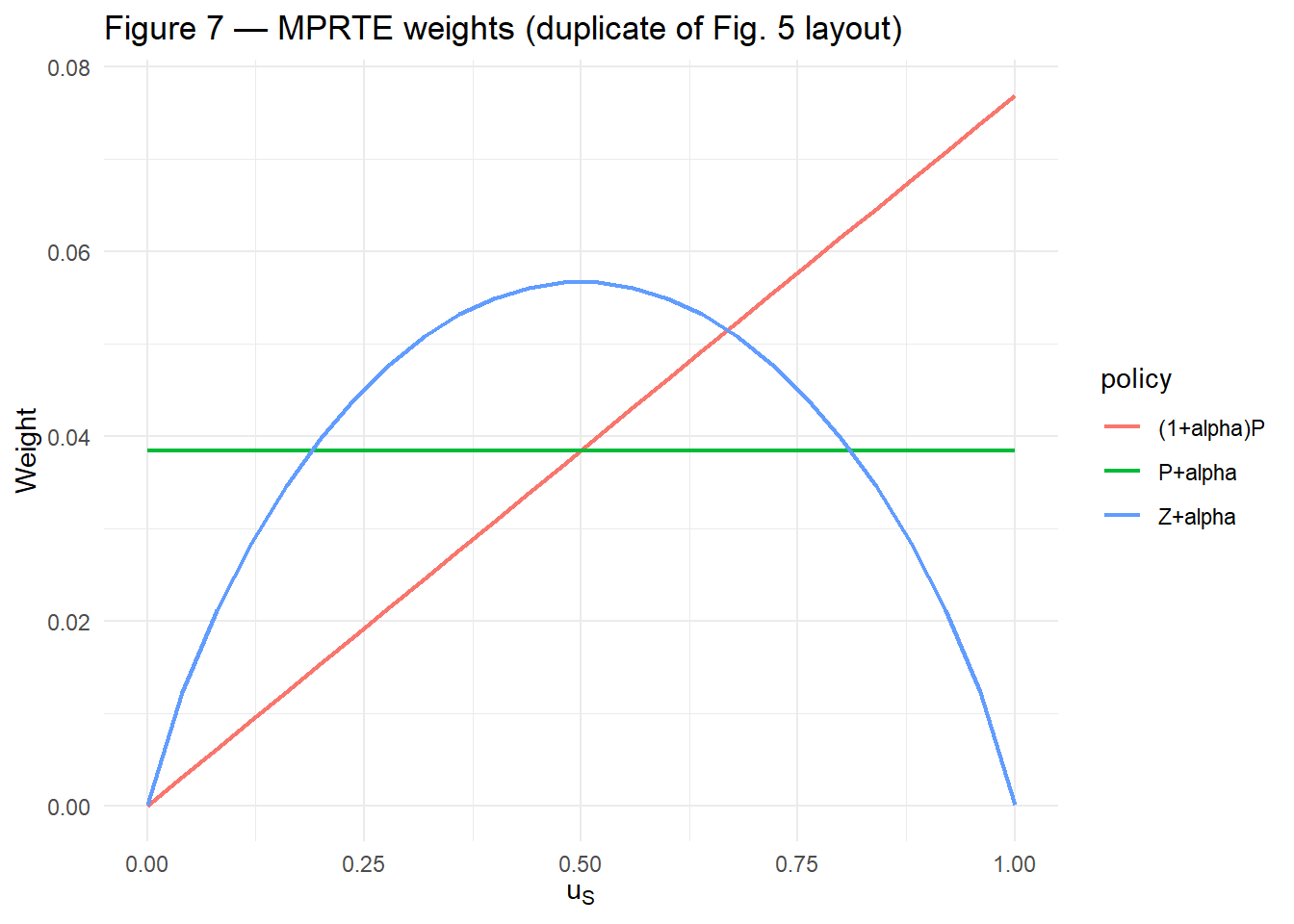
NoteReplication notes — Figure 7
- Procedure: Same weight layout as Figure 5 with alternate labeling (course placeholder for author Fig. 7).
- Status: Partial — same caveats as Figure 5.
- Caveats: Author Fig. 7 may differ in policy or trimming; confirm against the paper when comparing visually.
References
- Carneiro, P., Heckman, J. J., and Vytlacil, E. J. (2011). Estimating marginal returns to education. American Economic Review, 101(6), 2754–2781.
References
Carneiro, Pedro, James J. Heckman, and Edward Vytlacil. 2011. “Estimating Marginal Returns to Education.” The American Economic Review 101 (6): 2754–81. https://doi.org/10.1257/aer.101.6.2754.