Replication with R

Using Geographic Variation in College Proximity to Estimate the Return to Schooling

Author

Hu Huaping

Published

May 1, 2025

Introduction

This page replicates the empirical tables and Figure 1 in Card (1993) using the author’s proximity extract (nls.dat, $N = 3613$ for the 1976 cross-section). Walkthrough: replication guide. The analysis follows the modular R workflow used in Bound et al. (1995) and AK91.

Data: Rcode/proximity/nls.dat with column layout in code_bk.txt. SAS reference output: read1.lst (Table 2 col 1: ED76 = 0.0747, $N = 3010$).

Sample: Wage equations use men with valid 1976 log wages ($N = 3010$). Table 1 column (1) ($N = 5225$ full NLS-YM cohort) is not in the distributed data file; columns (2)–(3) are replicated.

File	Role
`card1993-data-prep.R`	`read_fwf`, variable construction, control vectors
`card1993-gt-quarto.R`	`gt` table formatting
`Table_I.R` – `Table_V.R`	Tables 1–5
`Figure_1.R`	Figure 1 — schooling by predicted-education quartile

Set rerun_script <- TRUE in the setup chunk to re-run all scripts and refresh .RData files.

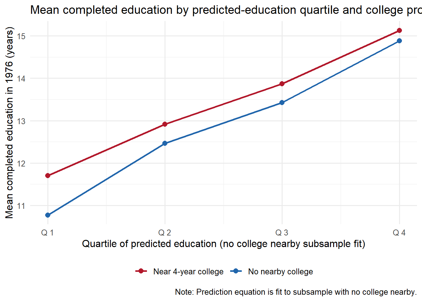
Figure 1 — College proximity and predicted schooling

Mean completed education by quartile of predicted schooling (fit on the no-nearby-college subsample) and 1966 college proximity.

Figure 1: (Figure 1)Mean completed education by predicted-education quartile and college proximity in 1966. Prediction equation is fit to subsample with no college nearby.

load(here("04-topics/rep-card1993/Rcode/Figure_1.RData"))
print(fig_summary)

# A tibble: 8 × 5
  pred_quartile nearc4 mean_ed     n nearc4_lab         
          <int>  <int>   <dbl> <int> <chr>              
1             1      0    10.8   358 No nearby college  
2             1      1    11.7   546 Near 4-year college
3             2      0    12.5   312 No nearby college  
4             2      1    12.9   591 Near 4-year college
5             3      0    13.4   254 No nearby college  
6             3      1    13.9   649 Near 4-year college
7             4      0    14.9   239 No nearby college  
8             4      1    15.1   664 Near 4-year college

print(paper_note)

# A tibble: 2 × 2
  metric                               value
  <chr>                                <dbl>
1 R2 prediction (no college subsample) 0.316
2 Lowest quartile gap (near - no)      0.935

Note: The prediction equation is fit on men who did not grow up near a 4-year college (nearc4 = 0); predicted schooling quartiles are then formed for the full sample. Replication $R^2 \approx 0.32$ (paper fn. 16: 0.30). Lowest-quartile gap in mean education (near vs. no college) is about 0.9–1.0 years here (paper: $\approx 1.1$ years).

Table 1 — Sample characteristics

Table 1: (Table 1) Sample characteristics for the overall sample and 1976 subsets of the National Longitudinal Survey of Young Men

	(1) Overall NLS-YM¹	(2) 1976 interview; valid education	(3) Valid wage & education
1. Age Distribution in 1966:
Age 14-15 (%)	—	25.3	25.5
Age 16-17	—	23.8	24.1
Age 18-20	—	24.1	24.7
Age 21-24	—	26.7	25.8
2. Regional Distribution in 1966:²
Northeast (%)	—	20.0	20.7
Midwest	—	26.3	26.0
South	—	41.3	41.4
West	—	12.5	11.9
3. Lived in SMSA 1966 (%)	—	64.3	65.0
4. Lived Near 4-year College in 1966 (%)	—	67.8	68.2
5. Family structure at Age 14:
Mother & Father (%)	—	79.2	78.9
Mother Only (%)	—	10.0	10.1
6. Average Parental Education
Mother's Education (yrs)	—	10.3	10.3
Father's Education (yrs)	—	10.0	10.0
7. Percent Black	—	23.0	23.4
8. Average score on KWW Test	—	33.5	33.5
9. Interviewed in 1976 (%)	—	100.0	100.0
10. Mean Education in 1976	—	13.2	13.3
11. Live in south in 1976 (%)	—	40.0	40.4
12. Sample size	5225	3613	3010
Notes: Means are based on all available valid observations in each subsample (Card, Table 1 notes).
¹ Column (1) shows published values for the original NLS-YM cohort (N = 5225). The proximity extract (`nls.dat`) contains only the 1976 cross-section; column (1) cannot be fully replicated from the distributed data file.
² Northeast = `reg661` + `reg662`; Midwest = `reg663` + `reg664`; West = `reg668` + `reg669`; South = `south66`.

load(here("04-topics/rep-card1993/Rcode/Table_I.RData"))
print(replication)

# A tibble: 1 × 9
  col2_n col3_n age_14_15_c2 age_14_15_c3 nearc4_c2 nearc4_c3 black_c2
   <int>  <int>        <dbl>        <dbl>     <dbl>     <dbl>    <dbl>
1   3613   3010         25.3         25.5      67.8      68.2     23.0
# ℹ 2 more variables: mean_ed_c2 <dbl>, mean_ed_c3 <dbl>

Table 2 — OLS log wage equations

Table 2: (Table 2) Estimated regression models for log hourly earnings (standard errors in parentheses)

stub	(1)	(2)	(3)	(4)	(5)
1. Education	0.074 (0.004)	0.075 (0.003)	0.073 (0.004)	0.074 (0.004)	0.073 (0.004)
2. Experience	0.084 (0.007)	0.085 (0.007)	0.085 (0.007)	0.085 (0.007)	0.085 (0.007)
3. Experience-squared /100	-0.224 (0.032)	-0.229 (0.032)	-0.230 (0.032)	-0.226 (0.032)	-0.229 (0.032)
4. Black Indicator	-0.190 (0.018)	-0.199 (0.018)	-0.194 (0.019)	-0.194 (0.019)	-0.189 (0.019)
5. Live in South	-0.125 (0.015)	-0.148 (0.026)	-0.146 (0.026)	-0.145 (0.026)	-0.146 (0.026)
6. Live in SMSA	0.161 (0.016)	0.136 (0.020)	0.136 (0.020)	0.137 (0.020)	0.138 (0.020)
7. Region in 1966 (8 indicators)	no	yes	yes	yes	yes
8. Live in SMSA in 1966	no	yes	yes	yes	yes
9. Parental education (years + missing indicators)¹	no	no	yes	yes	yes
10. Interacted parental education classes²	no	no	no	yes	yes
11. Family structure (2 indicators)³	no	no	no	no	yes
12. R-squared	0.291	0.300	0.301	0.303	0.304
13. F-test on family background variables	–	–	0.235	0.619	0.028
Notes: Standard errors in parentheses. Sample size is 3010. Dependent variable: log hourly wages in 1976 (mean 6.262, SD 0.444). Experience is `age76 − ed76 − 6`; experience-squared enters as (experience)$^2$/100 (SAS uses raw squared experience; coefficients differ by 100).
Replication: Column (1) education coefficient matches SAS `read1.lst` MODEL3 (`ED76 = 0.0747`). Row 13 incremental F-test p-values for columns (4)–(5) differ slightly from the paper (0.619 vs. 0.462; 0.028 vs. 0.165).
¹ Years of mother’s and father’s education plus indicators for imputed values (`nodaded`, `nomomed`).
² Eight interacted parental-education classes (`f1`–`f8` from `famed`).
³ Lived with both parents (`momdad14`); lived with single mother (`sinmom14`).

Table 3

load(here("04-topics/rep-card1993/Rcode/Table_II.RData"))
print(replication)

# A tibble: 5 × 5
    col     ed      se    r2       f
  <int>  <dbl>   <dbl> <dbl>   <dbl>
1     1 0.0740 0.00351 0.291 NA     
2     2 0.0747 0.00350 0.300 NA     
3     3 0.0733 0.00365 0.301  0.235 
4     4 0.0737 0.00368 0.303  0.619 
5     5 0.0726 0.00370 0.304  0.0282

print(paper_targets)

# A tibble: 5 × 5
    col    ed    se    r2      f
  <int> <dbl> <dbl> <dbl>  <dbl>
1     1 0.074 0.004 0.291 NA    
2     2 0.075 0.003 0.3   NA    
3     3 0.073 0.004 0.301  0.235
4     4 0.074 0.004 0.303  0.462
5     5 0.073 0.004 0.304  0.165

Table 3 — Reduced form and IV

Table 4: (Table 3) Reduced-form and structural estimates of education and earnings models (standard errors in parentheses)

stub	Reduced Education		Models: Earnings		Structural Models of Earnings
stub	(1)	(2)	(3)	(4)	(5)	(6)
Panel A: Treat experience and experience squared as exogenous
Live Near College in 1966	0.320 (0.088)	0.322 (0.083)	0.042 (0.018)	0.045 (0.018)	–	–
Education	–	–	–	–	0.132 (0.055)	0.140 (0.055)
Family Background variables¹	no	yes	no	yes	no	yes
Panel B: Treat experience and experience squared as endogenous²
Live Near College in 1966	0.382 (0.114)	0.365 (0.105)	0.047 (0.019)	0.048 (0.019)	–	–
Education	–	–	–	–	0.122 (0.046)	0.132 (0.049)
Family Background Variables¹	no	yes	no	yes	no	yes
Notes: Standard errors in parentheses. Sample size is 3010. Dependent variable in columns (1)–(2): completed education in 1976 (mean 13.263, SD 2.677). Dependent variable in columns (3)–(6): log hourly wages in 1976 (mean 6.262, SD 0.444). All models include black, 1976 South/SMSA, 1966 region/SMSA, experience and experience-squared.
Replication: Panel A IV columns (5)–(6) use Wald ratios of reduced-form coefficients. Panel B column (6) with full family background is the baseline IV specification for Table 4 row 1.
¹ Fourteen family-background controls: parental education (years and missing indicators), eight `famed` interaction classes, and two family-structure indicators (`card93_fb_full`).
² Experience and experience-squared are endogenous; instruments are `age76` and `age2` (= age76$^2$/100). Reduced-form equations use `ivreg` with experience instrumented by age.

load(here("04-topics/rep-card1993/Rcode/Table_III.RData"))
print(replication)

# A tibble: 4 × 5
  panel   col nearc_ed nearc_wage iv_ed
  <chr> <int>    <dbl>      <dbl> <dbl>
1 A         1    0.320     0.0421 0.132
2 A         2    0.322     0.0453 0.140
3 B         1    0.382     0.0467 0.122
4 B         2    0.365     0.0484 0.132

print(paper_targets)

# A tibble: 10 × 4
   panel   col metric     value
   <chr> <int> <chr>      <dbl>
 1 A         1 nearc_ed   0.32 
 2 A         2 nearc_ed   0.322
 3 A         1 nearc_wage 0.042
 4 A         2 nearc_wage 0.045
 5 A         5 iv_ed      0.132
 6 A         6 iv_ed      0.14 
 7 B         1 nearc_ed   0.382
 8 B         2 nearc_ed   0.365
 9 B         5 iv_ed      0.122
10 B         6 iv_ed      0.132

Table 4 — Robustness

Table 5: (Table 4) OLS and IV estimates of the return to education — alternative specifications (standard errors in parentheses)

stub	OLS Estimate	IV Estimate¹
1. Basic Specification (N = 3010)	0.073 (0.004)	0.132 (0.049)
2. Use 1978 Wages and Education (N = 2639 with 1978 data)	0.069 (0.004)	0.122 (0.062)
3. Include KWW Test Score (N = 2963 with valid KWW)	0.055 (0.004)	0.136 (0.078)
4. Include KWW; instrument KWW with IQ (N = 2040 with valid KWW and IQ)²	0.061 (0.005)	0.085 (0.013)
5. Use Proximity to Public College as instrument for education³	as in row 1	0.194 (0.059)
6. Use Proximities to 2-year and 4-year colleges as instruments for education⁴	as in row 1	0.117 (0.047)
7. Use Subsample Age 14-19 in 1966 (N = 2037)⁵	0.074 (0.006)	0.094 (0.064)
Notes: Dependent variable in rows 1 and 3–7: log hourly wages in 1976. Row 2: log hourly wages in 1978. Estimates are coefficients on the linear education term with black, 1976 South/SMSA, 1966 region/SMSA, experience and experience-squared, and fourteen family-background controls unless noted.
Replication: Row 2 uses all men with valid `lwage78` (N = 2639), not restricted to the N = 3010 wage subsample. Row 4 IV standard error is imprecise in this replication. Rows 5–6 OLS match row 1; only IV instruments differ.
¹ Education and experience are endogenous; instruments are `nearc4` (or alternatives noted below), `age76`, and `age2`, plus all exogenous controls. Row 1 matches Panel B, column (6) of Table 3.
² KWW enters the wage equation and is instrumented by IQ (`iq`); subsample with non-missing KWW and IQ.
³ Instrument for schooling is proximity to a public 4-year college (`nearc4a`).
⁴ Instruments are `nearc4` (4-year) and `nearc2` (2-year college proximity).
⁵ Subsample with `age66` $\leq$ 19 in 1966.

load(here("04-topics/rep-card1993/Rcode/Table_IV.RData"))
print(replication)

# A tibble: 7 × 6
    row     n    ols  ols_se     iv  iv_se
  <int> <int>  <dbl>   <dbl>  <dbl>  <dbl>
1     1  3010 0.0726 0.00370 0.132  0.0493
2     2  2639 0.0691 0.00406 0.122  0.0616
3     3  2963 0.0554 0.00440 0.136  0.0777
4     4  2040 0.0613 0.00549 0.0848 0.0126
5     5  3010 0.0726 0.00370 0.194  0.0591
6     6  3010 0.0726 0.00370 0.117  0.0472
7     7  2037 0.0745 0.00613 0.0944 0.0645

print(paper_targets)

# A tibble: 7 × 5
    row   ols ols_se    iv iv_se
  <int> <dbl>  <dbl> <dbl> <dbl>
1     1 0.073  0.006 0.132 0.049
2     2 0.066  0.006 0.117 0.061
3     3 0.055  0.004 0.136 0.078
4     4 0.061  0.005 0.089 0.085
5     5 0.073  0.006 0.194 0.059
6     6 0.073  0.006 0.117 0.047
7     7 0.076  0.006 0.094 0.064

Table 5 — Interaction IV

Table 6: (Table 5) IV estimates based on interaction of parental education and proximity to college (standard errors in parentheses)

stub	Reduced Form Models		Structural Models of Earnings
stub	Education	Earnings
Live Near College in 1966	0.228 (0.092)	0.031 (0.020)	0.001 (0.030)	0.013 (0.024)
Live College * Low Parental Education¹	0.436 (0.176)	0.065 (0.038)	–	–
Education²	–	–	0.149 (0.106)	0.097 (0.047)
Family Background Variables³	yes	yes	yes	yes
Notes: Standard errors in parentheses. Sample size is 3010. Dependent variable: log hourly wages in 1976 (mean 6.262, SD 0.444). All models include black, 1976 South/SMSA, 1966 region/SMSA, experience and experience-squared, and full family background. Experience is endogenous in structural columns; age and age-squared are instruments.
Replication: Reduced-form columns (1)–(2) use OLS; with endogenous experience, Panel B RF via `ivreg` gives slightly different point estimates. Direct effect of `nearc4` in columns (3)–(4) is small and imprecise.
¹ Interaction of an indicator for living near a 4-year college in 1966 with an indicator for both parents having less than high-school education (`lowfam = 1` if `famed = 9`; `nearc4_low = nearc4` $\times$ `lowfam`).
² Column (3): instrument for schooling is `nearc4_low`; coefficient is the Wald ratio of reduced-form earnings to schooling effects (paper: 0.093). Column (4): instruments are `nearc4` $\times$ `f1`–`nearc4` $\times$ `f8` (paper IV $\approx$ 0.097).
³ Fourteen controls (`card93_fb_full`): parental education (years and missing indicators), eight `famed` interaction classes, and two family-structure indicators at age 14.

load(here("04-topics/rep-card1993/Rcode/Table_V.RData"))
print(replication)

# A tibble: 8 × 4
    col var           estimate std.error
  <dbl> <chr>            <dbl>     <dbl>
1     1 nearc4_ed      0.228      0.0916
2     1 nearc4_low_ed  0.436      0.176 
3     2 nearc4_w       0.0312     0.0197
4     2 nearc4_low_w   0.0650     0.0379
5     3 iv_ed          0.149      0.106 
6     3 nearc4_direct  0.00105    0.0297
7     4 iv_ed          0.0971     0.0468
8     4 nearc4_direct  0.0129     0.0242

print(paper_targets)

# A tibble: 8 × 4
    col var           value    se
  <int> <chr>         <dbl> <dbl>
1     1 nearc4_ed     0.154 0.135
2     1 nearc4_low_ed 0.462 0.186
3     2 nearc4_w      0.029 0.024
4     2 nearc4_low_w  0.043 0.032
5     3 iv_ed         0.093 0.065
6     3 nearc4        0.015 0.029
7     4 iv_ed         0.097 0.048
8     4 nearc4        0.013 0.024