Ch17 Endogeneity and IV (Part A)

background-image: url("../pic/slide-front-page.jpg")
class: center,middle
count: false

# Advanced Econometrics III

## Simultaneous Equation Models (SEM)

### Hu Huaping (胡华平 )

### NWAFU (西北农林科技大学)

### School of Economics and Management (经济管理学院)

### huhuaping01 at hotmail.com

### 2026-06-04
<div>
<style type="text/css">.xaringan-extra-logo {
width: 110px;
height: 70px;
z-index: 0;
background-image: url(../pic/logo/nwafu-logo-circle-wb.png);
background-size: contain;
background-repeat: no-repeat;
position: absolute;
top:0.2em;left:1em;
}
</style>
<script>(function () {
  let tries = 0
  function addLogo () {
    if (typeof slideshow === 'undefined') {
      tries += 1
      if (tries < 10) {
        setTimeout(addLogo, 100)
      }
    } else {
      document.querySelectorAll('.remark-slide-content:not(.title-slide):not(.inverse):not(.hide_logo)')
        .forEach(function (slide) {
          const logo = document.createElement('div')
          logo.classList = 'xaringan-extra-logo'
          logo.href = null
          slide.appendChild(logo)
        })
    }
  }
  document.addEventListener('DOMContentLoaded', addLogo)
})()</script>
</div>

???

Good evening everyone. Welcome to my class.

I am teacher Hu Huaping.

Here is my email.

You can contact me when you have any questions with our course.

In this part, we will learn Simultaneous Equation Models together by using almost eight lessons.

---
count: false
class: center, middle, duke-orange,hide_logo

# Simultaneous Equation Models (SEM)

.large[

.red[Chapter 17. Endogeneity and Instrumental Variables]

Chapter 18. Why Should We Concern SEM ?

Chapter 19. What is the Identification Problem ?

Chapter 20. How to Estimate SEM ?

]

???

As you see this part contains four chapters.

Firstly, we will go through Chapter 17. Regressor Endogeneity problems and instrumental Variables solutions will be discussed in this chapter. Anyway, this chapter will be a good start for learning SEM.

The next three chapters focus closely on SEM. We will answer three important questions in turn.

In Chapter 18, we will know SEM is important in social science and it also brings new challenges to us.

Large SEM system always contains lots of parameters need to be solved and will face with the identification problems. We will give you guides and rules to check the SEM identification status in Chapter 19.

Finally, we will discuss different SEM estimation approaches in Chapter 20, including 2SLS, Three-stage least squares (3SLS) and full information maximum likelihood (FIML)  method.

---
layout: false
class: center, middle, duke-softblue,hide_logo
name: chapter17a

# Chapter 17. Endogeneity and Instumental Variables <br> (Part A)

[17.1 Definition and sources of endogeneity](#definition)

[17.2 Estimation problem with endogeneity](#problem)

[17.3 IV and the choices](#iv-choices)

[17.4 IV Identification: the lottery story](#iv-identification)

[17.5 IV Mechanics: RF, FS, and Wald](#iv-mechanics)

???
[source](https://web.sgh.waw.pl/~mrubas/AdvEcon/pdf/T2_Endogeneity.pdf)

So let us start the first chapter.

In this chapter:

- You will see how the method of **instrumental variables** (IV) can be used to solve the problem of **endogeneity** due to one or more regressors.

- Also we will learn the method of **two stage least squares** in section 17.6. 2SLS method is second in popularity only to ordinary least squares for estimating linear equations in econometrics.

- And some useful testing techniques will be introduced to check instrument validity and regressor endogeneity. These content will be uncovered in the last two sections.

---
layout: false
class: center, middle, duke-softblue,hide_logo
name: definition

## 17.1 Definition and sources of endogeneity

???
In this section we will talk about the definition of endogeneity and its main sources.

The story begins with the stochastic regressors.

---
layout: true

<div class="my-footer"><span>huhuaping@  <a href="#chapter17"> Chapter 17. Endogeneity and Instumental Variables  |</a>
&emsp;&emsp;&emsp;&emsp;&emsp;&emsp;&emsp;&emsp;&emsp;&emsp;&emsp;&emsp;&emsp;
<a href="#definition"> 17.1 Definition and source of endogeneity </a> </span></div>

---

### Think: How do we understand the world?

.page-font-18[

.fyi[

**Quick survey:** Which type of mental model does match you **mostly**? (A/B/C/D/E)
-  `$\Phi$` represents the **Truth** or **Causal Relationships**(Population Parameter), and
- `$X$` represents the **Sample Data**(Observed Data).
]

]

???

- Homo **apriorius**(pronounce: ah-pri-oh-re-us)
- Homo **pragmaticus**(pronounce: pra-gma-tic-us)
- Homo **frequentist**(pronounce: fre-kwen-tis-tus)
- Homo **sapiens**(pronounce: sa-pi-ens)
- Homo **bayesian**(pronounce: bay-see-an)

---

### Think: How do we understand the world?

.page-font-18[

- Homo **apriorius** (*illiterate villager*): Gut and lore—no data needed.
- Homo **pragmaticus** (*wage earner*): Grab the tool that works today.
- Homo **frequentist** (*white-collar*): Truth is what repeats forever.
- Homo **sapiens** (*Elon Musk*): Model the lever, test the design, scale the fix.
- Homo **bayesian** (*Einstein*): Theory first—then let evidence rewrite belief.

]

???

---

### Think: How do we understand the world?
<div class="figure">
<img src="../pic/chpt17-world-model-01.jpeg" alt="Objective world and mental models" width="792" />
<p class="caption">Objective world and mental models</p>
</div>

.footnote[
**Source**: Generated by AI with Google Nano Banana model
]

???

promotes-source: A split-screen illustration comparing three econometric approaches: Left side shows classical econometrics with OLS regression lines and parameter estimation, middle shows modern econometrics with causal inference experiments and policy evaluation, right side shows AI models with deep learning networks and pattern recognition. Include the central theme "How do we understand the world?" with mathematical symbols, data points, and network connections. Style: academic poster design with clear sections and professional typography.

---

### Think: How do we understand the world?

> **"All models are wrong, but some are useful."**
>  —— **George Box**

In the world of econometrics, we always face a fundamental question: **how to describe and predict complex economic phenomena using mathematical language?**

Now, we can compare three different "mental models" to help us understand the objective world:

.notes[
1. **Classical econometrics models**：find the "true" parameter or function form
2. **Modern econometrics models**：identify causal relationships and accurately predict the future
3. **AI (LLM) models**：learn data patterns and build world models
]

---

### Classical econometrics: observed data(0/4)
<div class="figure">
<img src="../pic/chpt17-curve-points.png" alt="A sample of data" width="693" />
<p class="caption">A sample of data</p>
</div>

---

### Classical econometrics: function A(1/4)
<div class="figure">
<img src="../pic/chpt17-curve-L.png" alt="Student A's view: a linear curve" width="675" />
<p class="caption">Student A's view: a linear curve</p>
</div>

---

### Classical econometrics: functon B(2/4)
<div class="figure">
<img src="../pic/chpt17-curve-U.png" alt="Student B's view: a parabolic curve" width="677" />
<p class="caption">Student B's view: a parabolic curve</p>
</div>

---

### Classical econometrics: function C(3/4)
<div class="figure">
<img src="../pic/chpt17-curve-S.png" alt="Student C's view: a S-shaped curve" width="665" />
<p class="caption">Student C's view: a S-shaped curve</p>
</div>

---

### Classical econometrics: Overview of the model

**Classical econometrics model** is a simplfied version of the objective world, and it is aimed to the **Truth** or **Causal Relationships**.

.fyi[
> **Classical econometrics model**  is a **Simple Model** but it is still an **World model** to help us understand the objective world.
]

`$$\begin{aligned}
Y_i &= \beta_1 + \beta_2 X_i + \epsilon_{1i}  &\text{(Linear Model)} \\
Y_i &= \beta_1 + \beta_2 X_i +\beta_3 X_i^2 + \epsilon_{2i} &\text{(Parabolic Model)} \\
Y_i &= \beta_1 + \beta_2 X_i +\beta_3 X_i^2 +\beta_4 X_i^3 + \epsilon_{3i} &\text{(S-shaped Model)}
\end{aligned}$$`

> In this point, we can think that the classical econometrics model is the same as the complex and mordern LLM models(AI models).

---

### Review: Gauss-Markov Theorem

.notes[
**Gauss-Markov Theorem**:

Under the CLRM assumptions(Classical Linear Regression Model Hypotheses) , the OLS estimator `$\hat{\Phi} \in \{\hat{\beta}_1, \hat{\beta}_2, \cdots, \hat{\sigma}^2\}$` is the .blue[BLUE] (the .blue[B]est .blue[L]inear .blue[U]nbiased .blue[E]stimator) of the population parameters `$\Phi \in \{\beta_1, \beta_2, \cdots, \sigma^2\}$`.
]

`$$\hat{\Phi} \overset{OLS}{\underset{CLRM}{\Longrightarrow}} \Phi \quad \text{is} \quad \color{#003366}{\text{BLUE}} \quad \text{(Best Linear Unbiased Estimator)}$$`

---

### Review: the CLRM assumptions

Let's revise the classic linear regression model   assumptions(CLRM):

- **A1**: The true model is
`$\boldsymbol{y= X \beta+\epsilon}$`.

- **A2**:
`$\forall i, E(\epsilon_i|X) = 0$` (conditional zero mean)  more about this later.

- **A3**:
`$Var(\epsilon|X) = E(\epsilon \epsilon^{\prime}|X) = \sigma^2I$` (identical conditional variance ).

- **A4**:
`$\boldsymbol{X}$` has full column rank.

- **A5**: (for inference purposes,
`$\boldsymbol{\epsilon} \sim  N(\boldsymbol{0}, σ^2\boldsymbol{I}))$`.

Under **A1-A4**(also namely **CLRM**), the OLS is **Gauss-Markov** efficient.

Under **A1-A5**, we donote **N-CLRM**.

???
we have discussed these assumptions before the class. And we denote the Gauss-Markov model assumption system as classical linear regression model (CLRM).

- **Assumption 1**: The  model is assumed to be true and be linear with parameters.

- **Assumption 2**: the disturbance term has conditional zero expectation. And we will relax this assumption later.

- **Assumption 3**: this means the conditional variance of disturcances is identity given X. the other way to express assumption 3 is that the  disturbance term is homoscedasticity['hɔməusi,dæs'tisəti].

- **Assumption 4**: The regressor matrix X has full column rank. Which means that none of the regressors is the perfect linear function on the rest of the regressors.

- **Assumption 5**: We will bring in the norm distribution assumption on the disburtance. This assumption aims for hypothesis testing purposes.

Joint with A2, A3, and A5, the disturbance is assumed to be normally identical independent distribution. We just write i.i.d for shortly.

With assumptions **A1-A4**, We note **CLRM**. Under CLRM the OLS is **Gauss-Markov** efficient. Which means under CLRM, when we use OLS method we will obtain the Best-Linear-unbiased estimators on the true parameters. [hand writing]

While, with assumptions **A1-A5**, we used to denote as N-CLRM. we can conduct kinds of inference and tests based on N-CLRM.

Now let us focus on assumption 2.

---

### Review: the A2 assumptions

For the population regression model(PRM):

`$$\begin{align}
Y_i &=  \beta_1 +\beta_2X_i + u_i && \text{(PRM)}
\end{align}$$`

- **CLRM A2** assumes that X is fixed (given) or independent of the error term. The regressors
`$X$` **are not** random variables. At this point, we can use the OLS method and get **BLUE**(Best Linear Unbiased Estimator).

`$$\begin{align}
Cov(X_i, u_i)= 0; \quad
E(X_i u_i)= 0
\end{align}$$`

- If the above A2 assumption is violated, the independent variable
`$X$` is related to the random disturbance term. In this case, OLS estimation will no longer get **BLUE**, and **instrumental variable method** (IV) should be used for estimation.

`$$\begin{align}
Cov(X_i, u_i) \neq 0 ; \quad
E(X_i u_i) \neq 0
\end{align}$$`

???

If A2 is violated, then the endogeneity problem arise.

Now we go head to define the endogenous variable.

Regardless of whether `$X_i$` and `$u_i$` are related, we can use the **IV method** to get **BLUE**.

---

###  Good model: random experiment

**Randomized controlled experiment **: Ideally, the value of the independent variable
`$X$` is randomly changed (refer to the **reason**), and then we look at the change in the dependent variable
`$Y$` (refer to the **result**).

`$$\boldsymbol{y = X \beta + u}$$`

- If
`$Y_i$` and
`$X_i$` does exist systematic relationship (linear relationship), then change
`$X_i$` causes the corresponding change of
`$Y_i$`.

- Any other random factors will be added to the random disturbance
`$u_i$`. The effect of the random disturbance on the change of `$Y_i$` should be **independent** to the effect of
`$X_i$` on the change of
`$Y_i$`.

---

###  Good model: exogenous regressors

**Exogenous regressors**: If independent variables
`$X_i$` is **perfectly random** (randomly assigned) as mentioned above , then they are called **exogenous regressor**. More precisely, they can be defined as:

.notes[

**Strictly Exogeneity**：

`$$E\left(u_{i} \mid X_{1}, \ldots, X_{N}\right)=E\left(u_{i} \mid \mathbf{x}\right)=0$$`

]

???

因为在**随机控制实验**，给定样本
`$i$`和样本
`$j$`，自变量的取值分别为
`$X_i$`和
`$X_j$`，它们应该是相互独立的。因此可以把上述假设进一步简化为：

> **同期外生性假设**(contemporaneously exogeneity)：
`$E(u_i|X_{i})=0, \text{for } i =1, \ldots,N$`。

**同期**表示的是在同样的时间点上，或所有的截面观测单位在某个时间上获得的观测。

大样本情况下OLS方法

在大样本情形下，上述**严格外生性假设**可以进一步转换为**同期不相关假设**：

- `$E(u_i)=0$`，而且

- `$\operatorname{cov}(X_i, u_i)=0$`

因为我们可以证明(证明略)，在大样本情况OLS方法下：

- `$E(u_i|X_{i})=0 \quad \Rightarrow \quad E(u_i)=0$`

- `$E(u_i|X_{i})=0 \quad \Rightarrow \quad \operatorname{cov}(X_i, u_i)=0$`

---

### Endogeneity: definition

We use the term **endogeneity** frequently in econometrics.

Also this concept is used broadly to describe any situation where a regressor is **correlated** with the error term.

- Assume that we have the bivariate linear model

`$$Y_{i}=\beta_{0}+\beta_{1} X_{i}+\epsilon_{i}$$`

- The explanatory variable
`$X$` is said to be **.red[En]dogenous** if it is correlated
with
`$\epsilon$`.

`$$\begin{align}
Cov(X_i, \epsilon_i) \neq 0 ; \quad
E(X_i \epsilon_i) \neq 0
\end{align}$$`

- And if
`$X$` is **uncorrelated** with
`$\epsilon$`, it is said to be **.red[Ex]ogenous**.

`$$\begin{align}
Cov(X_i, \epsilon_i) = 0 ; \quad
E(X_i \epsilon_i) = 0
\end{align}$$`

???
Next, we should ask what the sources of endogeneity come from.

---

### Endogeneity: sources

In applied econometrics, endogeneity usually arises in one of four ways:

- **Omitted variables**: when the model is set incorrectly.

- **Measurement errors** in the regressors.

- **Autocorrelation** of the error term in autoregressive models.

- **Simultaneity**: when
`$\boldsymbol{Y}$` and
`$\boldsymbol{X}$` are simultaneously determined, as in the supply/demand model (we will go to explain it in the next three chapter).

???

So, let us go through all of these four situations quickly.

---

### Source 1: Omitted variables

Suppose that the **"assumed true model"** for wage determination is:

`$$\begin{align}
Wage_{i}=\beta_{1}+\beta_{2} Edu_{i}+\beta_{3} Abl_{i}+\epsilon_{i}  \quad \text{(the assumed true model)}
\end{align}$$`

However, because the individual's **ability variable**(
`$Abl$`) is often not directly observed, so we often can't put it into the model, and build a **mis-specified model**.

`$$\begin{align}
Wage_{i}=\alpha_{1}+\alpha_{2} Edu_{i}+v_{i}  \quad \text{(the mis-specified model)}
\end{align}$$`

- Where **ability variable**(
`$Abl$`) is included in the new disturbance
`$v_i$`, and
`$v_{i}=\beta_{3} abl_{i}+u_{i}$`

- Obviously, in the mis-specified model, we ignore the **ability variable**(
`$Abl$`), while  variable **years of education**(
`$Edu$`) is actually related to it.

- So in the mis-specified  model,
`$cov(Edu_i, v_i) \neq 0$`, thus **years of education**(
`$Edu$`) may cause the endogenous problem.

???

why the variables are Omitted?  Because people run a model without considering the necessary  or important variables we should.

We will explain later that **Omission** of relevant variable will result in **inconsistent estimates** because **A2** is not hold.

Now, let us talk about the second source of endogeneity. the Measurement error in the regressors.

---

### Source A：Omitted variables (demo1) 1/4

Here we show a visual demonstration on this situation:

![](../pic/chpt11-endogeneity-ommit-sequence/chpt11-ommit-sequence-04.png)

<div class="box-A4">
  Assumed "TRUE MODEL":
</div>

---

### Source A：Omitted variables (demo1) 2/4

Here we show a visual demonstration on this situation:

![](../pic/chpt11-endogeneity-ommit-sequence/chpt11-ommit-sequence-03.png)

<div class="box-A4">
  Assumed "TRUE MODEL":
</div>

<div class="box-A3">
  "A's mis-specification MODEL":
</div>

---

### Source A：Omitted variables (demo1) 3/4

Here we show a visual demonstration on this situation:

![](../pic/chpt11-endogeneity-ommit-sequence/chpt11-ommit-sequence-02.png)

<div class="box-A4">
  Assumed "TRUE MODEL":
</div>

<div class="box-A3">
  "A's mis-specification MODEL":
</div>

---

### Source A：Omitted variables (demo1) 4/4

Here we show a visual demonstration on this situation:

![](../pic/chpt11-endogeneity-ommit-sequence/chpt11-ommit-sequence-01.png)

<div class="box-A4">
  Assumed "TRUE MODEL":
</div>

<div class="box-A3">
  "A's mis-specification MODEL":
</div>

<div class="box-A1">
  Omitted
`$\neq$` Disappeared
</div>

---

### Source 1：Omitted variables  (demo2)

An intuitive demonstration is show as follows:

![](../pic/chpt11-endogeneity-ommit-sequence/chpt11-ommit-sequence-part-05.png)

---

### Source 1：Omitted variables  (demo2)

An intuitive demonstration is show as follows:

![](../pic/chpt11-endogeneity-ommit-sequence/chpt11-ommit-sequence-part-04.png)

---

### Source 1：Omitted variables  (demo2)

An intuitive demonstration is show as follows:

![](../pic/chpt11-endogeneity-ommit-sequence/chpt11-ommit-sequence-part-03.png)

---

### Source 1：Omitted variables  (demo2)

An intuitive demonstration is show as follows:
![](../pic/chpt11-endogeneity-ommit-sequence/chpt11-ommit-sequence-part-02.png)

---

### Source 1：Omitted variables  (demo2)

An intuitive demonstration is show as follows:

![](../pic/chpt11-endogeneity-ommit-sequence/chpt11-ommit-sequence-part-01.png)

---

### Source B: Measurement errors

Again, let's consider the **"assumed true model"**:

`$$\begin{align}
Wage_{i}=\beta_{1}+\beta_{2} Edu_{i}+\beta_{3} Abl_{i}+\epsilon_{i}  \quad \text{(the assumed true model)}
\end{align}$$`

It is hard to observe individual's **ability variable**(
`$Abl$`), and somebody will instead to use the variable **IQ score**(
`$IQ_i$`), and construct the  mis-specified **"proxy variable" model**:

`$$\begin{align}
Wage_i=\alpha_{1}+\alpha_{2} Edu_i+\alpha_{3} IQ_i+v_i \quad \text{(the mis-specified model)}
\end{align}$$`

- It should exist stuffs (
`$Abl\_other_i$`) which the model does not include (due to the measurement error). So the measurement errors (
`$Abl\_other_i$`) will go to the disturbance term
`$v_i$` in the mis-specified model.

- And we know that measurement errors (
`$Abl\_other_i$`) will be correlated with the education variable. Thus `$cov(Edu_i, v_i) \neq 0$`, and the **education variable**(
`$Edu$`) may cause the endogenouse problem.

???

In practice, the observation value of a regressor is not accurate, in most time is only the "approximation".So there is **measurement error** in the regressor in our model.

---

### Source B: Measurement errors (demo 1) 1/4

Here we show a visual demonstration on this situation:

![](../pic/chpt11-endogeneity-measure-sequence/chpt11-measure-sequence-04.png)

<div class="box-B4">
  Assumed TRUE MODEL:
</div>

---

### Source B: Measurement errors (demo 1) 2/4

Here we show a visual demonstration on this situation:

![](../pic/chpt11-endogeneity-measure-sequence/chpt11-measure-sequence-03.png)

<div class="box-B4">
  Assumed TRUE MODEL:
</div>

<div class="box-B3">
  B's mis-specification MODEL:
</div>

---

### Source B: Measurement errors (demo 1) 3/4

Here we show a visual demonstration on this situation:

![](../pic/chpt11-endogeneity-measure-sequence/chpt11-measure-sequence-02.png)

<div class="box-B4">
  Assumed TRUE MODEL:
</div>

<div class="box-B3">
  B's mis-specification MODEL:
</div>

---

### Source B: Measurement errors (demo 1) 4/4

Here we show a visual demonstration on this situation:

![](../pic/chpt11-endogeneity-measure-sequence/chpt11-measure-sequence-01.png)

<div class="box-B4">
  Assumed TRUE MODEL:
</div>

<div class="box-B3">
  B's mis-specification MODEL:
</div>

<div class="box-B1">
  Measure Error
`$\neq$` Disappeared
</div>

---

### Source 2: Measurement errors (demo 2)

An intuitive demonstration is show as follows:

![](../pic/chpt11-endogeneity-measure-sequence/chpt11-measure-sequence-part-06.png)

---

### Source 2: Measurement errors (demo 2)

An intuitive demonstration is show as follows:

![](../pic/chpt11-endogeneity-measure-sequence/chpt11-measure-sequence-part-05.png)

---

### Source 2: Measurement errors (demo 2)

An intuitive demonstration is show as follows:

![](../pic/chpt11-endogeneity-measure-sequence/chpt11-measure-sequence-part-04.png)

---

### Source 2: Measurement errors (demo 2)

An intuitive demonstration is show as follows:

![](../pic/chpt11-endogeneity-measure-sequence/chpt11-measure-sequence-part-03.png)

---

### Source 2: Measurement errors (demo 2)

An intuitive demonstration is show as follows:

![](../pic/chpt11-endogeneity-measure-sequence/chpt11-measure-sequence-part-02.png)

---

### Source 2: Measurement errors (demo 2)

An intuitive demonstration is show as follows:

![](../pic/chpt11-endogeneity-measure-sequence/chpt11-measure-sequence-part-01.png)

---

### Source C: Autocorrelation

**Autoregressive model**: Lag variable of dependent variable(
`$Y_{t-1}, \ldots, Y_{t-p},\ldots$`) appears in the model as regressors.

`$$\begin{align}
Y_t=\beta_{1}+\beta_{2} Y_{t-1}+\beta_{3}X_t+u_t
\end{align}$$`

If the disturbance term determined following a first-order autocorrelation AR(1):

`$$\begin{align}
u_t=\rho u_{t-1}+ \epsilon_t
\end{align}$$`

Then, it is obvious that
`$cov(Y_{t-1}, u_{t-1}) \neq 0$` and
`$cov(Y_{t-1}, u_{t}) \neq 0$`.

Thus the **lag dependent variable**(
`$Y_{t-1}$`)  will cause the endogeneity problem in the **Autoregressive model**.

---

### Source C: Autocorrelation (demo 1) 1/4

Here we show a visual demonstration on this situation:

![](../pic/chpt11-endogeneity-ar-sequence/chpt11-ar-sequence-04.png)

<div class="box-C4">
  Assumed TRUE MODEL: AR(1)
</div>

---

### Source C: Autocorrelation (demo 1) 2/4

Here we show a visual demonstration on this situation:

![](../pic/chpt11-endogeneity-ar-sequence/chpt11-ar-sequence-03.png)

<div class="box-C4">
  Assumed TRUE MODEL: AR(1)
</div>

<div class="box-C31">
  (main model)
</div>

<div class="box-C32">
  (auxiliary model)
</div>

---

### Source C: Autocorrelation (demo 1) 3/4

Here we show a visual demonstration on this situation:

![](../pic/chpt11-endogeneity-ar-sequence/chpt11-ar-sequence-02.png)

<div class="box-C4">
  Assumed TRUE MODEL: AR(1)
</div>

<div class="box-C31">
  (main model)
</div>

<div class="box-C32">
  (auxiliary model)
</div>

---

### Source C: Autocorrelation (demo 1) 4/4

Here we show a visual demonstration on this situation:

![](../pic/chpt11-endogeneity-ar-sequence/chpt11-ar-sequence-01.png)

<div class="box-C4">
  Assumed TRUE MODEL: AR(1)
</div>

<div class="box-C31">
  (main model)
</div>

<div class="box-C32">
  (auxiliary model)
</div>

<div class="box-C1">
  Hidden
`$\neq$` Disappeared
</div>

---

### Source C: Autocorrelation (demo 2) 1/5

An intuitive demonstration is show as follows:

![](../pic/chpt11-endogeneity-ar-sequence/chpt11-ar-sequence-part2-05.png)

<div class="box-Cs5">
  (main model)
</div>

---

### Source C:  Autocorrelation (demo 2) 2/5

An intuitive demonstration is show as follows:

![](../pic/chpt11-endogeneity-ar-sequence/chpt11-ar-sequence-part2-04.png)

<div class="box-Cs5">
  (main model)
</div>

<div class="box-Cs4">
  (derived model)
</div>

---

### Source C:  Autocorrelation (demo 2) 3/5

An intuitive demonstration is show as follows: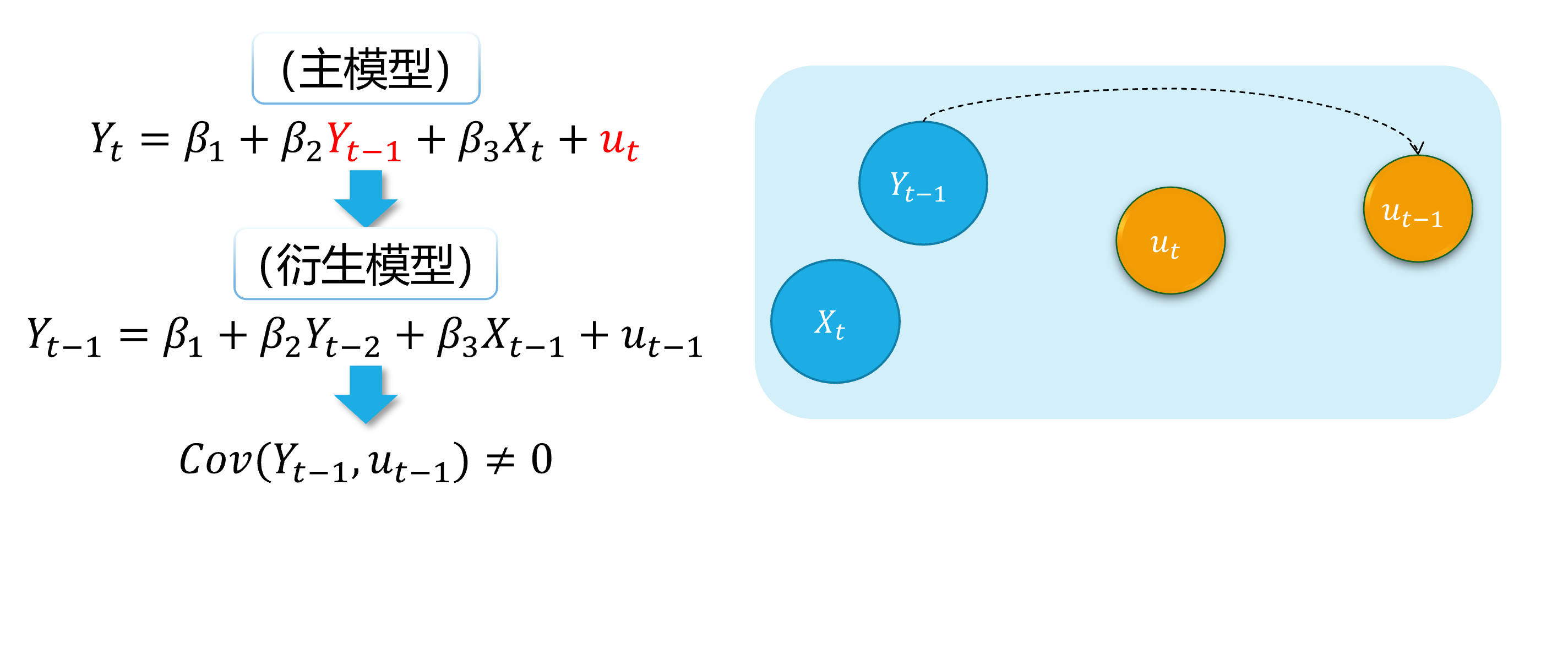

![](../pic/chpt11-endogeneity-ar-sequence/chpt11-ar-sequence-part2-03.png)

<div class="box-Cs5">
  (main model)
</div>

<div class="box-Cs4">
  (derived model)
</div>

---

### Source C:  Autocorrelation (demo 2) 4/5

An intuitive demonstration is show as follows: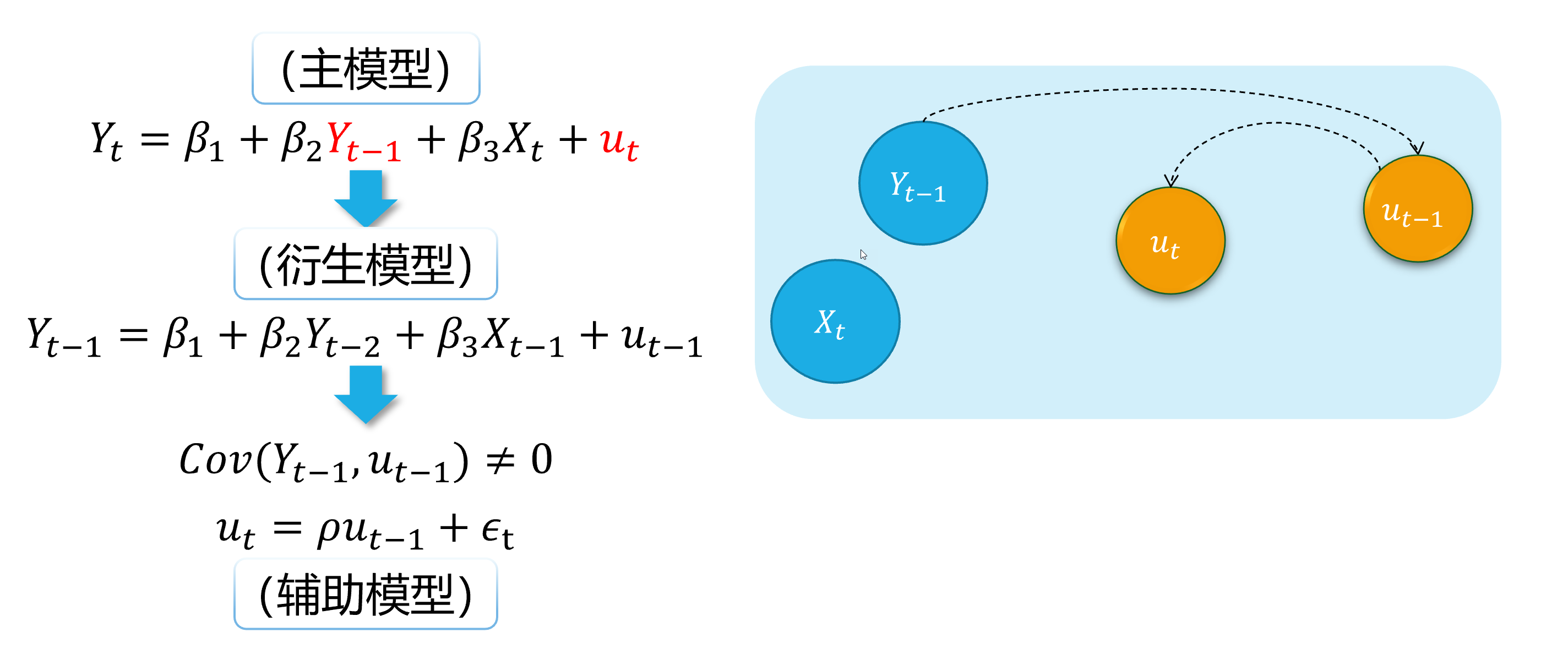

![](../pic/chpt11-endogeneity-ar-sequence/chpt11-ar-sequence-part2-02.png)

<div class="box-Cs5">
  (main model)
</div>

<div class="box-Cs4">
  (derived model)
</div>

<div class="box-Cs2">
 (auxiliary model)
</div>

---

### Source C:  Autocorrelation (demo 2) 5/5

An intuitive demonstration is show as follows: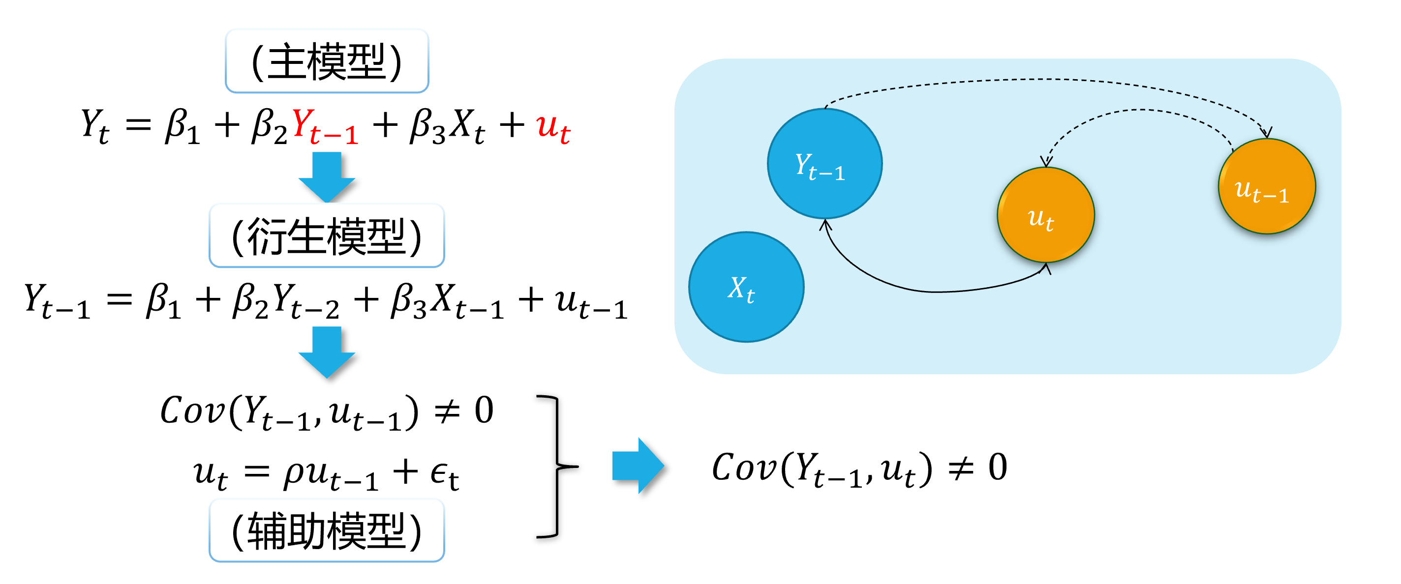

![](../pic/chpt11-endogeneity-ar-sequence/chpt11-ar-sequence-part2-01.png)

<div class="box-Cs5">
  (main model)
</div>

<div class="box-Cs4">
  (derived model)
</div>

<div class="box-Cs2">
 (auxiliary model)
</div>

---

### Source D: Simultaneity

For the equations system of supply and demand:

`$$\begin{cases}
  \begin{align}
    \text { Demand: } & Q_{i}=\alpha_{1}+\alpha_{2} P_{i}+u_{d i} \\
    \text { Supply: } & Q_{i}=\beta_{1}+\beta_{2} P_{i} + u_{s i}
  \end{align}
\end{cases}$$`

As we all know, because of the price
`$P_i$` will both affect supply and the demand `$Q_i$`, And vice versa. There is a feedback cycle mechanism in this system.

So, we can get
`$cov(P_i, u_{di}) \neq 0$`, and
`$cov(P_i, u_{si}) \neq 0$`, which will cause the endogenous problem finally.

???
/ˌsɪmltəˈneɪət/

---

### Source D: Simultaneity (demo 1) 1/4

Here we show a visual demonstration on this situation: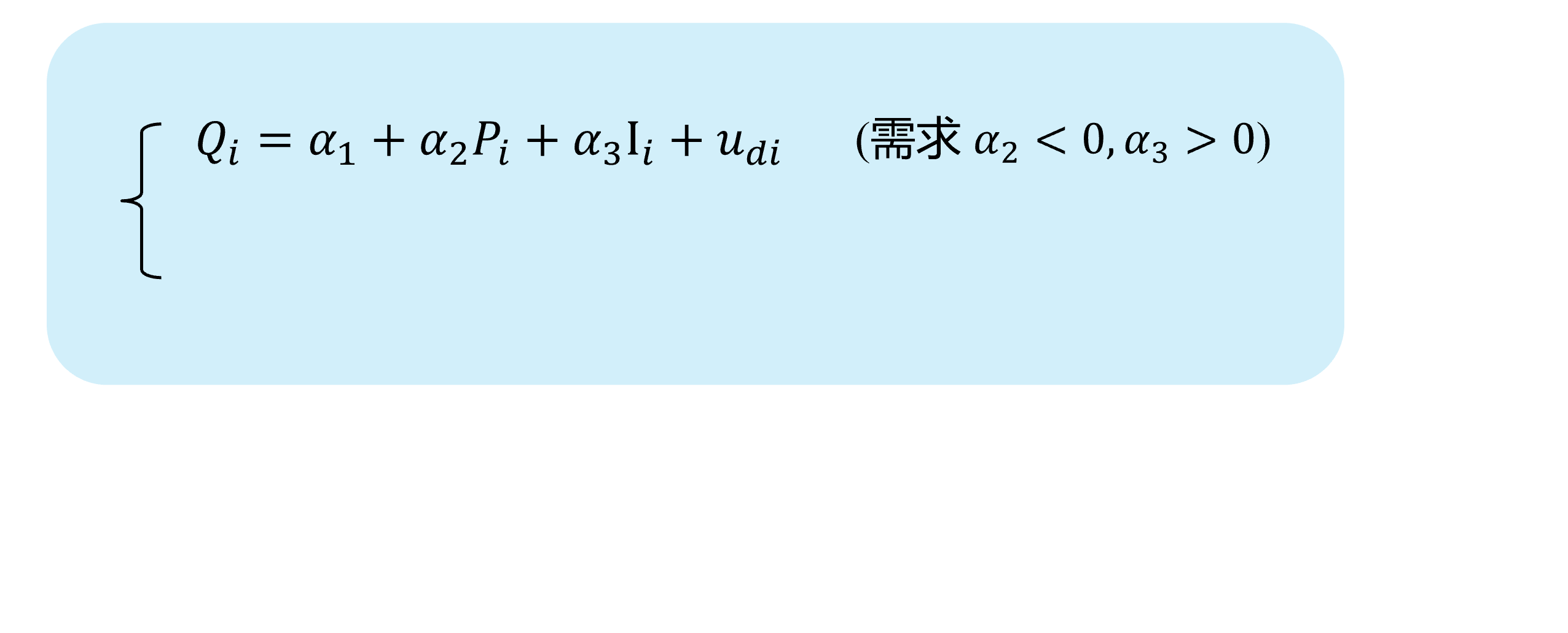

![](../pic/chpt11-endogeneity-sem-sequence/chpt11-sem-sequence-04.png)

<div class="box-D4">
  (Demand
</div>

---

### Source D: Simultaneity (demo 1) 2/4

Here we show a visual demonstration on this situation: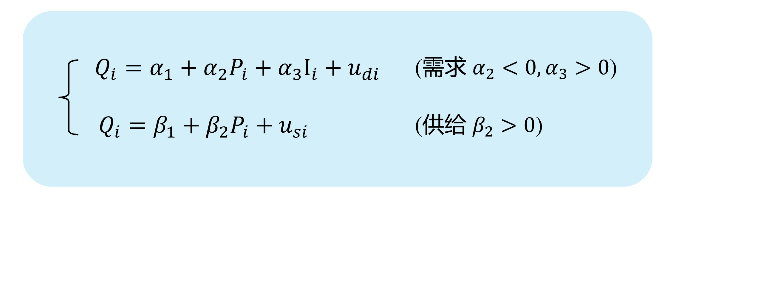

![](../pic/chpt11-endogeneity-sem-sequence/chpt11-sem-sequence-03.png)

<div class="box-D4">
  (Demand
</div>

<div class="box-D3">
  (Supply
</div>

---

### Source D: Simultaneity (demo 1) 3/4

Here we show a visual demonstration on this situation: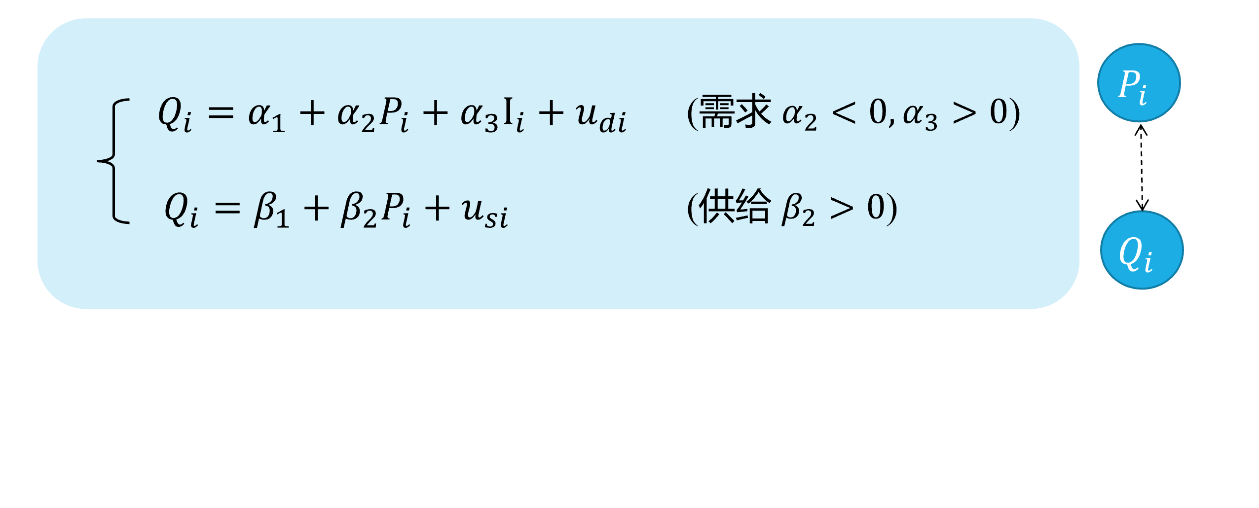

![](../pic/chpt11-endogeneity-sem-sequence/chpt11-sem-sequence-02.png)

<div class="box-D4">
  (Demand
</div>

<div class="box-D3">
  (Supply
</div>

---

### Source D: Simultaneity (demo 1) 4/4

Here we show a visual demonstration on this situation: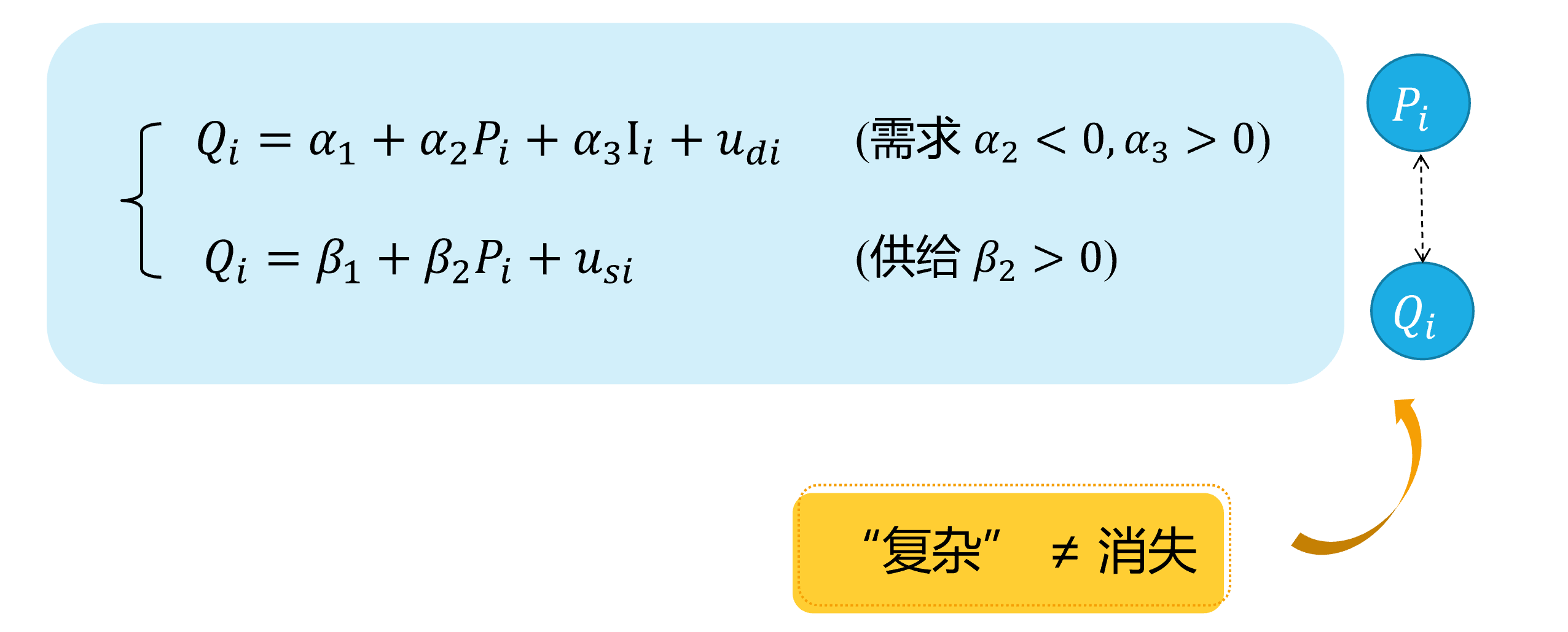

![](../pic/chpt11-endogeneity-sem-sequence/chpt11-sem-sequence-01.png)

<div class="box-D4">
  (Demand
</div>

<div class="box-D3">
  (Supply
</div>

<div class="box-D1">
  Hidden
`$\neq$` Disappeared
</div>

---

### Source D: Simultaneity (demo 2) 1/5

An intuitive demonstration is show as follows: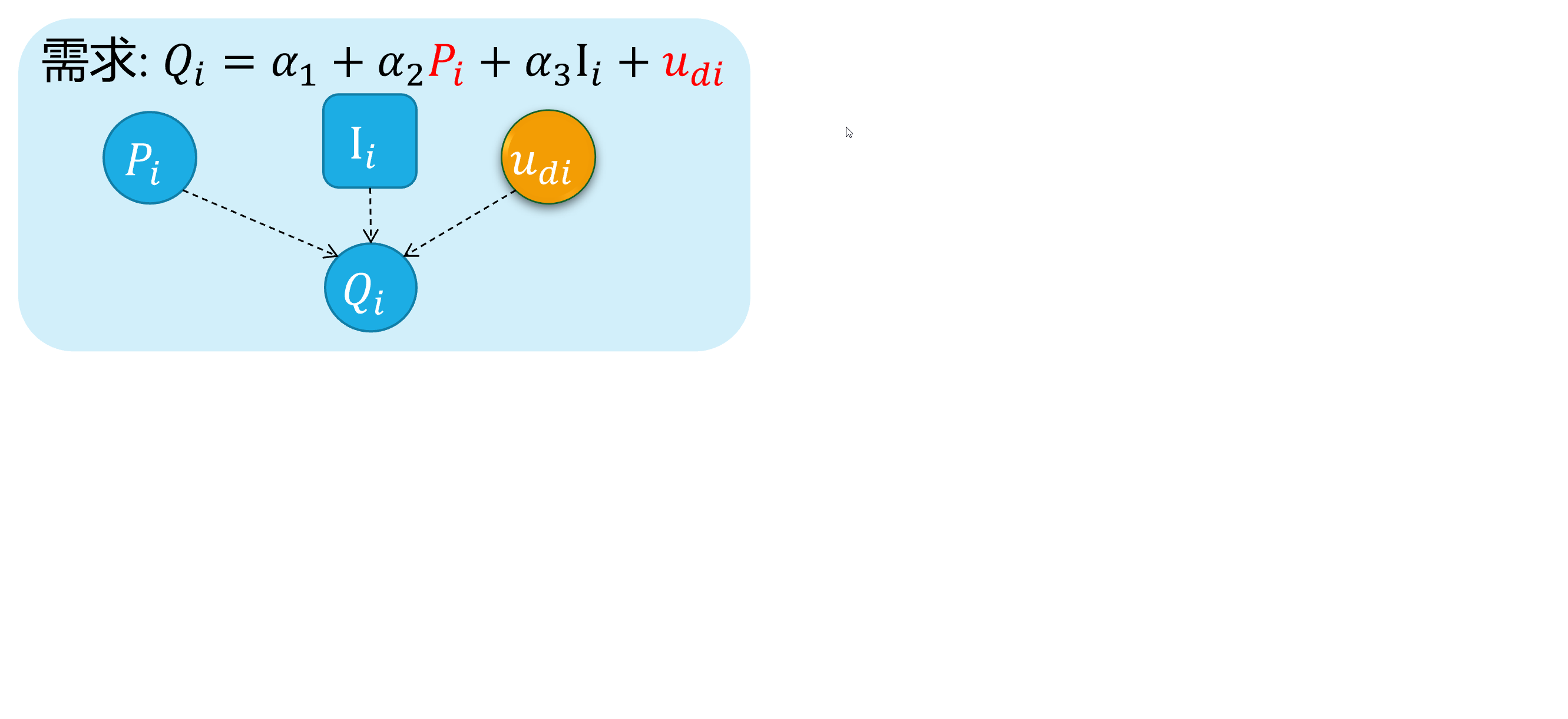

![](../pic/chpt11-endogeneity-sem-sequence/chpt11-sem-sequence-part-05.png)

---

### Source D: Simultaneity (demo 2) 2/5

An intuitive demonstration is show as follows: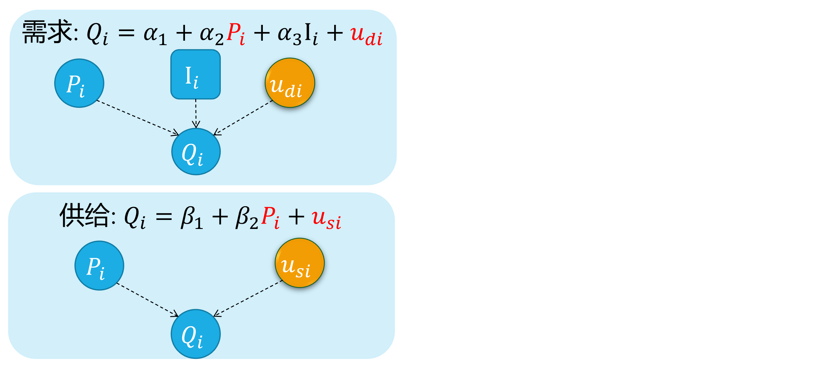

![](../pic/chpt11-endogeneity-sem-sequence/chpt11-sem-sequence-part-04.png)

---

### Source D: Simultaneity (demo 2) 3/5

An intuitive demonstration is show as follows: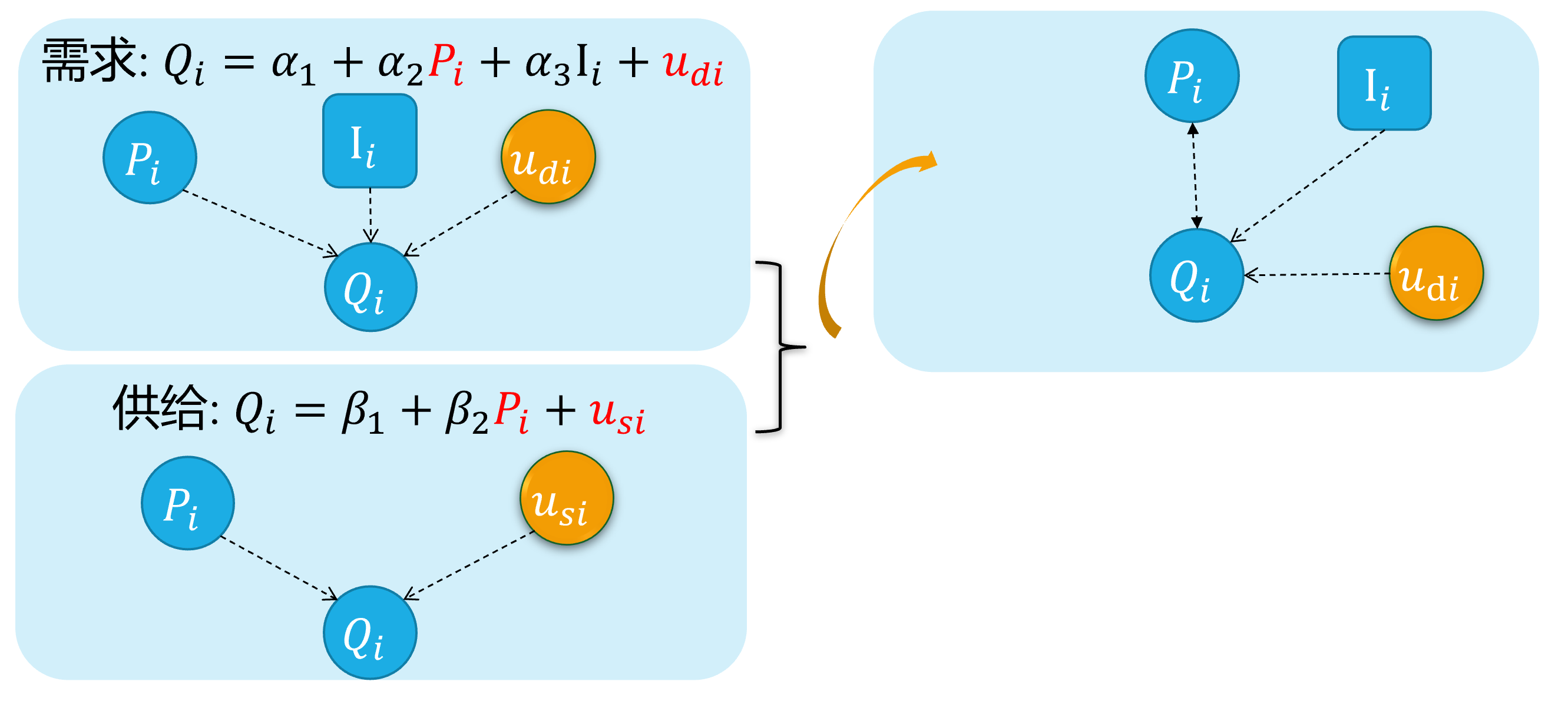

![](../pic/chpt11-endogeneity-sem-sequence/chpt11-sem-sequence-part-03.png)

---

### Source D: Simultaneity (demo 2) 4/5

An intuitive demonstration is show as follows: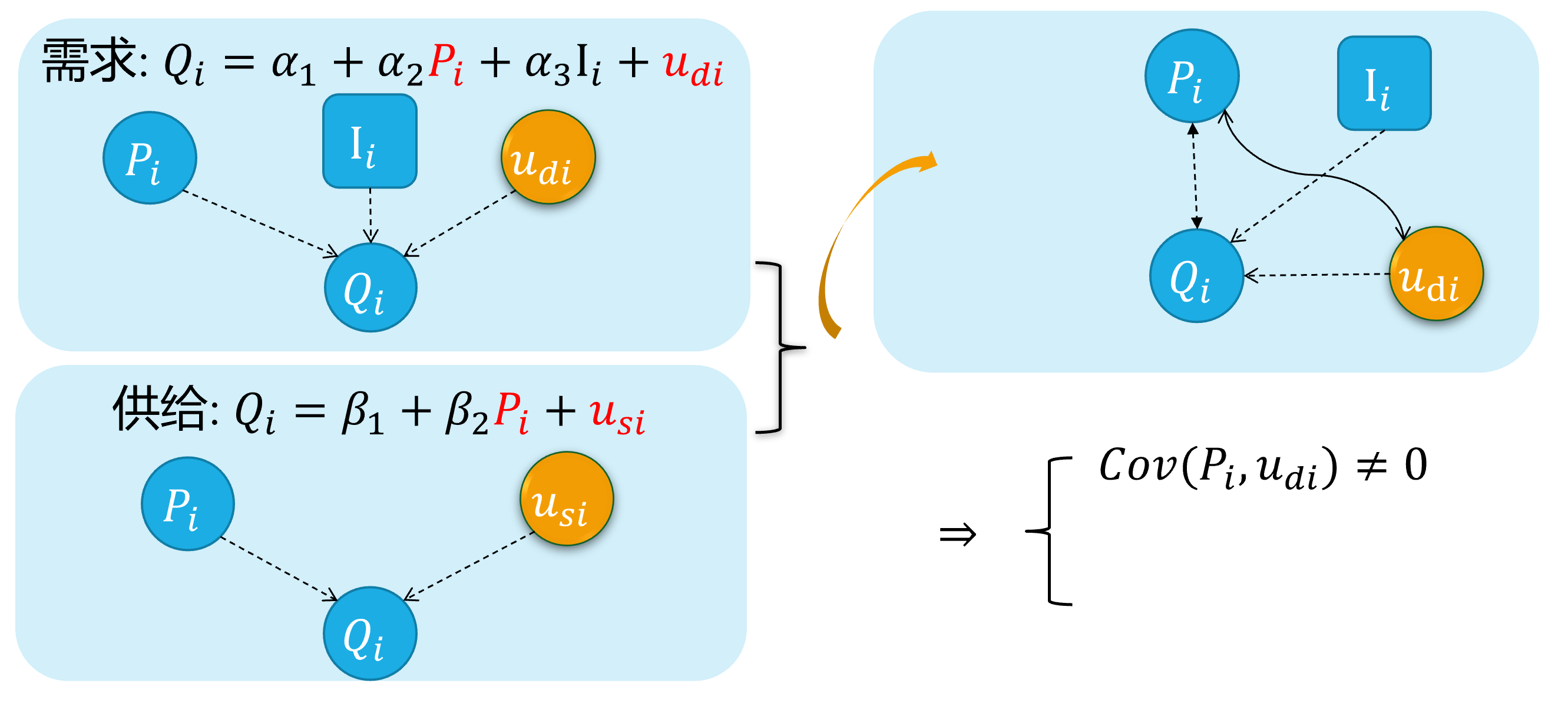

![](../pic/chpt11-endogeneity-sem-sequence/chpt11-sem-sequence-part-02.png)

---

### Source D: Simultaneity (demo 2) 5/5

An intuitive demonstration is show as follows: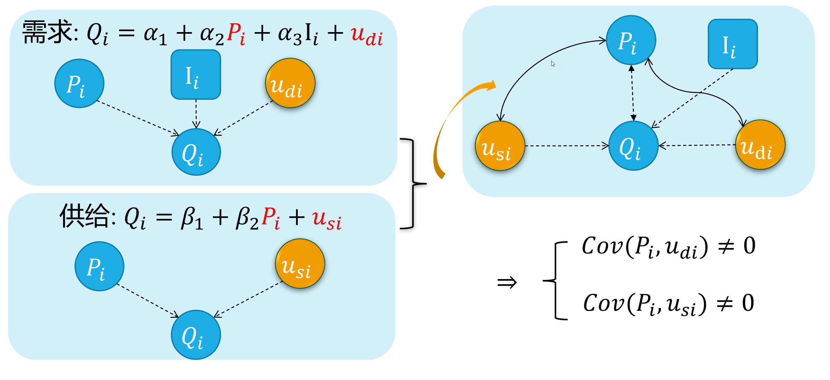

![](../pic/chpt11-endogeneity-sem-sequence/chpt11-sem-sequence-part-01.png)

---

layout: false
class: center, middle, duke-softblue,hide_logo
name: problem

## 17.2 Estimation problem with endogeneity

???
The question is what will happen on OLS estimators with model contains endogenous regressors.

So, let us illustrate these estimation problems in detail in this section.

we will discuss along two different situations.

---
layout: true

<div class="my-footer"><span>huhuaping@   <a href="#chapter17"> Chapter 17. Endogeneity and Instumental Variables  |</a> &emsp;&emsp;&emsp;&emsp;&emsp;&emsp;&emsp;&emsp;&emsp;&emsp;&emsp;&emsp;&emsp; <a href="#problem"> 17.2 Estimation problem with endogeneity </a></span></div>

---

### Inconsistent estimates with measurement error

Consider the simple regression model:

`$$Y_{i}=\beta_{0}+\beta_{1} X_{i}+\epsilon_{i} \quad \text{(1)}$$`

We would like to measure the effect of the variable `$X$` on `$Y$`, but we can observe only an imperfect measure of it (i.e. a **proxy variable**), which is

`$$X^{\ast}_{i}=X_{i} - v_{i} \quad \text{(2)}$$`

Where
`$v_i$` is a random disturbance with mean 0 and variance `$\sigma_{v}^{2}$`.

Further, let's assume that `$X_i, \epsilon_i$` and `$v_i$` are **pairwise independent**.

???

In the second situation, OLS estimators will be also inconsistent with measurement error on regressors.

---

### Inconsistent estimates with measurement error

Given the assumed true model (1):

`$$\begin{aligned}
Y_{i} &=\beta_{0}+\beta_{1} X_{i}+\epsilon_{i} && \text{ eq(1) assumed true model }
\end{aligned}$$`

with the proxy variable `$X^{\ast}_i$`, we may use the error specified model (4):

`$$\begin{aligned}
X^{\ast}_i &= X_i - v_i && \text{ eq(2) proxy variable }\\
X_i &= X^{\ast}_i + v_i && \text{ eq(3)}\\
Y_{i} &=\beta_{0}+\beta_{1} X^{\ast}_{i}+u_{i} && \text{ eq(4) error specified model}
\end{aligned}$$`

We can substitute eq (3) into the model (1) to obtain eq(5)

`$$\begin{aligned}
Y_{i} = \beta_{0}+\beta_{1} X_{i}^{*}+\epsilon_{i}
&= \beta_{0}+\beta_{1}\left(X^{\ast}_{i} + v_{i}\right)+\epsilon_{i} \\
&= \beta_{0}+\beta_{1} X^{\ast}_{i}+\left(\epsilon_{i} + \beta_{1} v_{i}\right) \quad \text{(5)}
\end{aligned}$$`

which means `$u_{i}=\left(\epsilon_{i}+\beta_{1} v_{i}\right)$` in the error specified model. As we know, the OLS consistent estimator of `$\beta_{1}$` in the last equation .red[**requires**] `$\operatorname{Cov}\left(X^{\ast}_{i}, u_{i}\right)= 0$`.

???
For simplicity, we just replace the `$X_i$` in the assumed true model 1, with the proxy variable `$X^{\ast}_i$`, and get the error specified model 4.

Meanwhile the measurement error will fall into the composite error term `$u_i$`. As you see.

---

### Inconsistent estimates with measurement error

Note that
`$E\left(u_{i}\right)=E\left(\epsilon_{i} +\beta_{1} v_{i}\right)=E\left(\epsilon_{i}\right)+\beta_{1} E\left(v_{i}\right)=0$`

However,

`$$\begin{aligned}
  \operatorname{Cov}\left(X^{\ast}_{i}, u_{i}\right)
    &= E\left[\left(X^{\ast}_{i}-E\left(X^{\ast}_{i}\right)\right)\left(u_{i}-E\left(u_{i}\right)\right)\right] \\
    &= E\left(X^{\ast}_{i} u_{i}\right) \\
    &= E\left[\left(X_{i}-v_{i}\right)\left(\epsilon_{i} +\beta_{1} v_{i}\right)\right] \\
    &= E\left[X_{i} \epsilon_{i}+\beta_{1} X_{i} v_{i}- v_{i}\epsilon_{i}- \beta_{1} v_{i}^{2}\right]
       \leftarrow \quad \text{(pairwise independent)} \\
    &= -E\left(\beta_{1} v_{i}^{2}\right) \\
    &= -\beta_{1} \operatorname{Var}\left(v_{i}\right) \\
    &= -\beta_{1} \sigma_{v_i}^{2} \neq 0
\end{aligned}$$`

Thus,
`$X$` in model (4) is .red[**endogenous**] and we expect the OLS estimator of
`$\beta_{1}$` to be **inconsistent**.

???

So far as we know, both omitted variable(s) and error measurement will cause endogeneity, and result in violation of A2.

Let us sum up all these cases in general.

---

### OLS estimation: Violation of A2

In general, when **A2** is violated, we expect OLS estimates to be **biased**:

The OLS estimators of `$\hat{\beta}$` is

`$$\begin{align}
\widehat{\beta} &=\beta+\left(X^{\prime} X\right)^{-1} X^{\prime} \epsilon && \text{(6)}
\end{align}$$`

and we can take expectation on both sides.

`$$\begin{aligned}
  E(\widehat{\beta}) &= \beta+E\left(\left(X^{\prime} X\right)^{-1} X^{\prime} \epsilon\right) \\
  &= \beta+E\left(E\left(\left(X^{\prime} X\right)^{-1} X^{\prime} \epsilon \mid X\right)\right) \\
  &= \beta+E\left(\left(X^{\prime} X\right)^{-1} X^{\prime} E(\epsilon \mid X)\right) \neq \beta
\end{aligned}$$`

If **A2**
`$E(\epsilon | X) = 0$` is violated, which means
`$E(\epsilon | X) \neq 0$`, the OLS estimator is **biased**.

???

The result will show that the OLS estimator is not equal to its true parameter if **A2** is violated.

> Here, you should know that the value take expectation on conditional expectation is equal to unconditional expectation.

---

### OLS estimation: consistency

Let's see under what conditions we can establish consistency.

`$$\begin{aligned}
  p \lim \widehat{\beta} &= \beta+p \lim \left(\left(X^{\prime} X\right)^{-1} X^{\prime} \epsilon\right) \\
  &= \beta+p \lim \left(\left(\frac{1}{n} X^{\prime} X\right)^{-1} \frac{1}{n} X^{\prime} \epsilon\right) \\
  &= \beta+p \lim \left(\frac{1}{n} X^{\prime} X\right)^{-1} \times p \lim \left(\frac{1}{n} X^{\prime} \epsilon\right)
\end{aligned}$$`

By the WLLN (Weak Law of Large Numbers)

`$$\frac{1}{n} X^{\prime} \epsilon=\frac{1}{n} \sum_{i=1}^{n} X_{i} \epsilon_{i} \xrightarrow{p} E\left(X_{i} \epsilon_{i}\right)$$`

Hence
`$\widehat{\beta}$` is consistent if
`$E\left(X_{i} \epsilon_{i}\right)=0$` for all `$i$`. The condition
`$E\left(X_{i} \epsilon_{i}\right)=0$` is more likely to be satisfied than A2
`$E(\epsilon | X) = 0$`. Thus, a large class of estimators that cannot be proved to be **unbiased** are **consistent**.

???

Let's see under what conditions we can establish consistency.

We can take the probability limits on both sides of equation (6).

we will derive that the probability limits of this part will equal to expectation of `$X_i$` times `$\epsilon_i$`

We have dived deeply with theory evidence.

Now, I will show you an example.

---

### Wage example: the origin model

Consider the following "error specified" wage model:

`$$\begin{align}
lwage_i = \beta_1 +\beta_2educ_i + \beta_3exper_i +\beta_4expersq_i + e_i
\end{align}$$`

The difficulty with this model is that the error term may include some unobserved attributes, such as personal **ability**, that determine both wage and education.

In other words, the independent variable  **educ**  is correlated with the error term. And it is endogenous variable.

> **Note**:

> We will use **years of schooling** as the proxy variable of **educ** in practice, and it surely bring in error measurement issues as we have mentioned.

???

Consider the following error specified wage model, which the logarithmic (ˌlɒɡəˈrɪðmɪk) wage is the function of education,labor market experience and its quadratic term.

As what we have discussed before. The difficulty with this model is that the error term may include some unobserved attributes, such as personal **ability**, that determine both wage and education.

> There is one more thing we should remind. We will use **years of schooling** as the proxy variable of **educ** in practice, and it surely bring in error measurement issues as we have mentioned.

Let us show all variables of our dataset.

---

### Wage example: All variables in dataset

With data set `wooldridge::mroz`, researchers were interest in the return to education for married women.

<div class="datatables html-widget html-fill-item" id="htmlwidget-9d725b296593dfcf7ae1" style="width:100%;height:auto;"></div>
<script type="application/json" data-for="htmlwidget-9d725b296593dfcf7ae1">{"x":{"filter":"none","vertical":false,"extensions":["Buttons"],"caption":"<caption>Variables and Labels<\/caption>","data":[["1","2","3","4","5","6","7","8","9","10","11","12","13","14","15","16","17","18","19","20","21","22"],[1,2,3,4,5,6,7,8,9,10,11,12,13,14,15,16,17,18,19,20,21,22],["educ","exper","expersq","fatheduc","lwage","motheduc","wage","age","city","faminc","hours","husage","huseduc","hushrs","huswage","inlf","kidsge6","kidslt6","mtr","nwifeinc","repwage","unem"],[" years of schooling"," actual labor mkt exper"," exper^2"," father's years of schooling"," log(wage)"," mother's years of schooling"," est. wage from earn, hrs"," woman's age in yrs"," =1 if live in SMSA"," family income, 1975"," hours worked, 1975"," husband's age"," husband's years of schooling"," hours worked by husband, 1975"," husband's hourly wage, 1975"," =1 if in lab frce, 1975","  kids 6-18","  kids  under 6 years"," fed. marg. tax rte facing woman"," (faminc - wage*hours)/1000"," rep. wage at interview in 1976"," unem. rate in county of resid."]],"container":"<table class=\"display\">\n  <thead>\n    <tr>\n      <th> <\/th>\n      <th>index<\/th>\n      <th>vars<\/th>\n      <th>labels<\/th>\n    <\/tr>\n  <\/thead>\n<\/table>","options":{"dom":"Btip","pageLength":6,"buttons":["copy","csv","excel"],"initComplete":"function(settings, json) {\n$(this.api().table().header()).css({'background-color': '#517fb9', 'color': '#fff'});\n}","columnDefs":[{"className":"dt-right","targets":1},{"orderable":false,"targets":0},{"name":" ","targets":0},{"name":"index","targets":1},{"name":"vars","targets":2},{"name":"labels","targets":3}],"order":[],"autoWidth":false,"orderClasses":false,"lengthMenu":[6,10,25,50,100]},"callback":"function(table) {\n$(\"button.buttons-copy\").css(\"background\",\"yellow\");\n                $(\"button.buttons-csv\").css(\"background\",\"orange\");\n                $(\"button.buttons-excel\").css(\"background\",\"#a88d32\");\n                $(\"button.dt-button\").css(\"padding\",\"0.2em 0.2em\");\n                $(\"button.dt-button\").css(\"font-size\",\"0.6em\");\n                $(\"button.dt-button\").css(\"margin-right\",\"0.2em\");\n                $(\"button.dt-button\").css(\"margin-bottom\",\"0.1em\");\n                $(\"button.dt-button\").css(\"line-height\",\"1em\");\n                return table;\n}"},"evals":["options.initComplete","callback"],"jsHooks":[]}</script>

???

Other variables include father education, mother education, which are both measured by schooling years, etc (ɪt ˈsetərə).

---

### Wage example: Raw dataset

<div class="datatables html-widget html-fill-item" id="htmlwidget-223da7232337c9492819" style="width:100%;height:auto;"></div>
<script type="application/json" data-for="htmlwidget-223da7232337c9492819">{"x":{"filter":"none","vertical":false,"extensions":["Buttons"],"caption":"<caption>dataset n=(428)<\/caption>","data":[["1","2","3","4","5","6","7","8","9","10","11","12","13","14","15","16","17","18","19","20","21","22","23","24","25","26","27","28","29","30","31","32","33","34","35","36","37","38","39","40","41","42","43","44","45","46","47","48","49","50","51","52","53","54","55","56","57","58","59","60","61","62","63","64","65","66","67","68","69","70","71","72","73","74","75","76","77","78","79","80","81","82","83","84","85","86","87","88","89","90","91","92","93","94","95","96","97","98","99","100","101","102","103","104","105","106","107","108","109","110","111","112","113","114","115","116","117","118","119","120","121","122","123","124","125","126","127","128","129","130","131","132","133","134","135","136","137","138","139","140","141","142","143","144","145","146","147","148","149","150","151","152","153","154","155","156","157","158","159","160","161","162","163","164","165","166","167","168","169","170","171","172","173","174","175","176","177","178","179","180","181","182","183","184","185","186","187","188","189","190","191","192","193","194","195","196","197","198","199","200","201","202","203","204","205","206","207","208","209","210","211","212","213","214","215","216","217","218","219","220","221","222","223","224","225","226","227","228","229","230","231","232","233","234","235","236","237","238","239","240","241","242","243","244","245","246","247","248","249","250","251","252","253","254","255","256","257","258","259","260","261","262","263","264","265","266","267","268","269","270","271","272","273","274","275","276","277","278","279","280","281","282","283","284","285","286","287","288","289","290","291","292","293","294","295","296","297","298","299","300","301","302","303","304","305","306","307","308","309","310","311","312","313","314","315","316","317","318","319","320","321","322","323","324","325","326","327","328","329","330","331","332","333","334","335","336","337","338","339","340","341","342","343","344","345","346","347","348","349","350","351","352","353","354","355","356","357","358","359","360","361","362","363","364","365","366","367","368","369","370","371","372","373","374","375","376","377","378","379","380","381","382","383","384","385","386","387","388","389","390","391","392","393","394","395","396","397","398","399","400","401","402","403","404","405","406","407","408","409","410","411","412","413","414","415","416","417","418","419","420","421","422","423","424","425","426","427","428"],[1,2,3,4,5,6,7,8,9,10,11,12,13,14,15,16,17,18,19,20,21,22,23,24,25,26,27,28,29,30,31,32,33,34,35,36,37,38,39,40,41,42,43,44,45,46,47,48,49,50,51,52,53,54,55,56,57,58,59,60,61,62,63,64,65,66,67,68,69,70,71,72,73,74,75,76,77,78,79,80,81,82,83,84,85,86,87,88,89,90,91,92,93,94,95,96,97,98,99,100,101,102,103,104,105,106,107,108,109,110,111,112,113,114,115,116,117,118,119,120,121,122,123,124,125,126,127,128,129,130,131,132,133,134,135,136,137,138,139,140,141,142,143,144,145,146,147,148,149,150,151,152,153,154,155,156,157,158,159,160,161,162,163,164,165,166,167,168,169,170,171,172,173,174,175,176,177,178,179,180,181,182,183,184,185,186,187,188,189,190,191,192,193,194,195,196,197,198,199,200,201,202,203,204,205,206,207,208,209,210,211,212,213,214,215,216,217,218,219,220,221,222,223,224,225,226,227,228,229,230,231,232,233,234,235,236,237,238,239,240,241,242,243,244,245,246,247,248,249,250,251,252,253,254,255,256,257,258,259,260,261,262,263,264,265,266,267,268,269,270,271,272,273,274,275,276,277,278,279,280,281,282,283,284,285,286,287,288,289,290,291,292,293,294,295,296,297,298,299,300,301,302,303,304,305,306,307,308,309,310,311,312,313,314,315,316,317,318,319,320,321,322,323,324,325,326,327,328,329,330,331,332,333,334,335,336,337,338,339,340,341,342,343,344,345,346,347,348,349,350,351,352,353,354,355,356,357,358,359,360,361,362,363,364,365,366,367,368,369,370,371,372,373,374,375,376,377,378,379,380,381,382,383,384,385,386,387,388,389,390,391,392,393,394,395,396,397,398,399,400,401,402,403,404,405,406,407,408,409,410,411,412,413,414,415,416,417,418,419,420,421,422,423,424,425,426,427,428],[1.210153698921204,0.3285121023654938,1.514137744903564,0.09212332218885422,1.524272203445435,1.556480050086975,2.120259523391724,2.059634208679199,0.7543363571166992,1.544899344444275,1.401921629905701,1.524272203445435,0.7339532375335693,0.8183690905570984,1.302831172943115,0.2980283796787262,1.167609572410583,1.643839359283447,0.6931471824645996,2.021931648254395,1.254247546195984,1.272957682609558,1.178655028343201,1.178655028343201,0.7675586938858032,1.331811785697937,1.386294364929199,1.553269624710083,1.981814861297607,1.769360423088074,0.430807888507843,0.8997548222541809,1.766629695892334,1.272957682609558,1.336788892745972,0.9017048478126526,0.8651236891746521,1.511847138404846,1.72602915763855,2.683142423629761,0.9852942824363708,1.365938544273376,0.9450336694717407,1.512376189231873,0.6931471824645996,1.244788408279419,0.7011649012565613,1.519863247871399,0.8209685683250427,0.9698315262794495,0.828508198261261,0.09430964291095734,0.1625438928604126,0.4700036346912384,0.6292484402656555,1.397160172462463,2.265443801879883,2.084541082382202,1.525838851928711,0.762160062789917,1.48160457611084,1.262826442718506,0.9996755719184875,1.832581520080566,2.479307651519775,1.279015302658081,1.937935590744019,1.070452809333801,1.12392258644104,1.321755886077881,1.744999766349792,1.301743626594543,1.641866445541382,2.107020139694214,1.46706759929657,1.605811357498169,-1.029739379882812,1.08768618106842,0,0.9382086992263794,-0.1505903750658035,0,1.073670506477356,1.265848398208618,0.4863689839839935,2.120259523391724,1.129852533340454,0.9932518005371094,1.658627986907959,0.3474121987819672,1.568324208259583,0.5108456015586853,0.1148454323410988,-0.6931471824645996,-0.3364522755146027,1.028225541114807,1.58068859577179,0.5558946132659912,0.9014207124710083,0.8843045830726624,0.4282045960426331,1.058415055274963,0.8783395886421204,1.654908299446106,1.321755886077881,0.3285121023654938,1.386294364929199,1.172884583473206,1.224187135696411,0.2876570820808411,2.23026180267334,1.504077434539795,1.531152009963989,1.375157594680786,1.760268807411194,-0.6931471824645996,1.406489133834839,1.791759490966797,1.299292087554932,1.351003885269165,1.016280889511108,1.075343608856201,1.478964686393738,1.689486742019653,2.288597822189331,-1.822631120681763,-0.9607651829719543,1.290994167327881,0.8648711442947388,1.540452122688293,0.6162121295928955,1.648658633232117,1.193498134613037,2.143976211547852,0.7244035601615906,0.9416075348854065,0.7827593684196472,1.832581520080566,1.203962802886963,1.491644859313965,1.892132639884949,2.130894899368286,1.48060405254364,0.8943313360214233,0.2025325447320938,0.4855078160762787,1.098612308502197,1.553269624710083,0.1215979680418968,2.001804351806641,1.495036602020264,0.9052298069000244,0.6325475573539734,1.386294364929199,2.102913856506348,1.959643959999084,0.5108456015586853,1.236923933029175,1.443312525749207,1.021659255027771,0.6361534595489502,1.616453289985657,0.2231435477733612,1.049807071685791,1.415051937103271,0.5753766298294067,2.60668158531189,1.517914533615112,0.7550415992736816,1.094972372055054,0.9421143531799316,1.724942803382874,1.031546115875244,0.474369078874588,0.8109301924705505,0.7092666029930115,1.710549473762512,0.4602688848972321,1.331811785697937,1.098612308502197,2.157998561859131,1.437581300735474,1.544899344444275,1.41059672832489,3.218875885009766,0.9681618809700012,1.791759490966797,1.688729524612427,-0.4091719686985016,0.2231435477733612,0.8221558332443237,1.24170196056366,1.427124381065369,1.497097492218018,0.5596157908439636,1.300028204917908,1.884429812431335,0.9555113911628723,1.582087278366089,1.755614042282104,1.513103246688843,2.251891613006592,2.364432334899902,0.1053504794836044,1.399728775024414,0.988462507724762,1.090647339820862,1.154614448547363,1.266947627067566,2.885191679000854,1.228880047798157,1.203962802886963,1.357380270957947,0.8377236127853394,0.5369611382484436,0.7487238049507141,2.295872688293457,1.107803225517273,0.6208452582359314,-2.054163694381714,1.892012000083923,1.729724526405334,0.4693784117698669,0.9808416962623596,2.069492340087891,1.675188183784485,1.386294364929199,1.799214959144592,1.832581520080566,1.090647339820862,1.443123579025269,1.250360131263733,1.602312564849854,1.018558502197266,1.297053217887878,1.685194492340088,-0.4209848940372467,1.562094688415527,2.146527528762817,2.347462892532349,0.9698315262794495,1.924146413803101,1.62672758102417,-0.03926072642207146,1.460148692131042,1.955393552780151,0.9263598918914795,2.066191673278809,1.422843217849731,2.10103178024292,2.261461019515991,0.7013137936592102,2.031012535095215,1.162369251251221,0.4700036346912384,1.41059672832489,0.3930551111698151,1.290994167327881,0,0.9571254849433899,0.5596157908439636,1.568615913391113,1.710187911987305,1.41059672832489,0.2231435477733612,0.5108456015586853,1.332392454147339,0.8601858615875244,2.322779893875122,1.91959547996521,1.976106762886047,0.8954347372055054,0.18123759329319,0.4953058362007141,0.5777924060821533,1.07881772518158,1.603198528289795,0.6208452582359314,2.083894014358521,1.379169106483459,1.112383723258972,1.067121624946594,1.118806958198547,1.588541030883789,1.390311241149902,1.714806437492371,0.2010615319013596,0.9872710108757019,0.9835006594657898,2.233170747756958,1.143617510795593,-0.6113829016685486,2.153052091598511,1.299837350845337,0.8409204483032227,1.058484435081482,1.152658462524414,1.293575882911682,1.832581520080566,2.327180147171021,1.166146278381348,2.034993171691895,0.6792510747909546,1.547136902809143,0.7530185580253601,0.8472836017608643,0.8711259961128235,0.2282504737377167,0.08965782821178436,1.321755886077881,1.196101903915405,1.636118769645691,1.892012000083923,1.518308997154236,2.472159147262573,1.321755886077881,1.473641037940979,1.369478821754456,1.203962802886963,1.198729157447815,1.270209908485413,0.4700036346912384,0.7999816536903381,1.565945625305176,1.758978009223938,0.858025848865509,0.6931471824645996,0.6418538689613342,1.633740186691284,1.703747630119324,1.844004034996033,1.966118812561035,0.8649974465370178,0.9333052039146423,0.7792331576347351,0.9555113911628723,1.316247344017029,1.475906491279602,1.491397261619568,1.455750465393066,0.5108456015586853,1.180438041687012,1.688489437103271,0.7907274961471558,1.401798605918884,-0.4335560202598572,1.683171510696411,-1.766676664352417,3.155595064163208,2.259521007537842,1.306926369667053,0.7984976768493652,0.5590441823005676,0.1479026228189468,1.944494843482971,1.378337860107422,3.064745187759399,-0.7419173121452332,0.7657003998756409,0.619392991065979,1.465452075004578,2.18925952911377,1.021659255027771,0.9770094752311707,0.9162907600402832,2.905096054077148,-0.1996711939573288,0.6931471824645996,2.733392953872681,1.868334650993347,2.120259523391724,1.515193223953247,0.9146093130111694,1.499556064605713,0.803077220916748,0.7280316352844238,0.5164099931716919,1.22644829750061,0.9162907600402832,1.376471281051636,1.828974962234497,1.368283152580261,1.064710736274719,1.406489133834839,1.047318935394287,1.948093414306641,1.078001379966736,0.6539384722709656,1.927891612052917,1.361027836799622,0.6931471824645996,1.604686617851257,0.1839036494493484,3.113515377044678,1.926829218864441,1.2701256275177,0.6826927065849304,1.68106997013092,0.5562959909439087,1.628220438957214,0.9162907600402832,1.341558456420898,0,1.122231245040894,0.5401707887649536,1.391505718231201,1.697173953056335,3.218875885009766,0.871167778968811,1.167329549789429,1.216987729072571,0.5753766298294067,1.151615738868713,0.9942512512207031,0.5263249278068542,-1.543182134628296,1.91204309463501,0.554287314414978,0.9162907600402832,1.500939130783081,0.9446837902069092,1.241268634796143,1.564984321594238,0.8380264639854431,1.668857097625732,1.769428610801697,1.22644829750061,1.406489133834839],[12,12,12,12,14,12,16,12,12,12,12,11,12,12,10,11,12,12,12,12,16,12,13,12,12,17,12,12,17,12,11,16,13,12,16,11,12,10,14,17,12,12,16,12,12,12,16,12,12,12,12,12,12,8,10,16,14,17,14,12,14,12,8,12,12,8,17,12,12,12,12,12,9,10,12,12,12,17,15,12,6,14,12,14,9,17,13,9,15,12,12,12,12,12,12,12,12,13,12,13,12,12,12,16,12,13,11,12,12,12,17,14,16,17,12,11,12,12,17,10,13,11,12,16,17,12,16,12,16,8,12,12,12,13,11,12,12,14,12,12,12,17,14,12,9,12,12,12,14,16,17,15,12,16,17,17,12,16,13,12,11,16,14,16,12,9,17,14,12,12,11,12,12,10,12,5,17,11,12,12,14,11,12,14,12,10,16,13,12,12,12,11,12,9,13,12,12,12,13,16,12,16,17,12,12,9,12,12,13,12,12,12,12,10,12,16,12,11,12,10,12,12,12,12,16,17,12,17,12,12,12,8,12,13,12,12,8,12,17,17,12,13,12,12,12,12,9,10,12,16,13,8,16,13,12,11,13,12,12,10,12,17,15,16,10,11,12,12,14,16,14,8,7,12,12,14,12,12,12,14,16,12,12,12,13,13,10,12,12,12,12,14,17,10,9,12,12,16,12,17,12,17,11,16,11,13,11,8,11,12,10,17,12,12,17,14,12,12,12,12,12,12,9,10,12,12,12,12,12,17,12,17,12,10,12,12,12,12,12,12,16,13,13,12,16,17,12,14,12,17,12,14,12,12,17,16,16,12,9,12,12,16,14,12,12,11,12,16,17,17,14,12,14,12,10,12,13,16,12,7,16,14,12,10,12,16,10,12,14,12,6,15,12,17,14,13,6,16,14,15,14,8,14,12,12,12,12,12,12,8,12,17,12,12,14,13,17,8,12,11,12,12,17,10,12,13,12,12],[14,5,15,6,7,33,11,35,24,21,15,14,0,14,6,9,20,6,23,9,5,11,18,15,4,21,31,9,7,7,32,11,16,14,27,0,17,28,24,11,1,14,6,10,6,4,10,22,16,6,12,32,15,17,34,9,37,10,35,6,19,10,11,15,12,12,14,11,9,24,12,13,29,11,13,19,2,24,9,6,22,30,10,6,29,29,36,19,8,13,16,11,15,6,13,22,24,2,6,2,2,14,9,11,9,6,19,26,19,3,7,28,13,9,15,20,29,9,1,8,19,23,3,13,8,17,4,15,11,7,0,0,10,8,2,4,6,18,3,22,33,28,23,27,11,6,11,14,17,17,14,11,7,8,6,8,4,25,24,11,19,9,19,14,22,6,23,15,6,11,2,22,10,14,12,9,13,18,8,11,9,9,14,9,2,12,15,11,7,9,19,11,8,13,4,7,19,14,14,3,9,7,7,14,29,19,14,16,10,12,24,6,9,14,26,7,4,15,23,1,29,9,6,11,17,6,7,2,24,4,11,25,11,2,19,7,2,20,10,19,17,12,11,6,10,4,2,13,21,9,4,2,19,4,9,14,6,24,1,13,3,10,16,9,19,4,10,5,7,3,38,16,13,1,7,15,10,2,19,25,25,7,15,11,25,19,4,14,19,18,14,11,4,29,21,24,19,31,28,15,27,13,4,10,8,4,18,3,11,8,10,33,19,35,21,7,18,4,12,16,14,3,1,27,12,6,9,2,6,9,16,22,26,11,11,15,13,6,20,17,8,13,15,14,14,6,24,10,2,9,23,12,8,16,10,7,19,2,9,14,9,16,7,6,22,9,9,14,17,12,13,8,10,16,1,6,4,8,4,15,7,14,16,15,23,19,4,12,12,25,14,14,11,7,18,4,37,13,14,17,5,2,0,3,21,20,19,4,19,11,14,8,13,24,1,1,3,4,21,10,13,9,14,2,21,22,14,7],[196,25,225,36,49,1089,121,1225,576,441,225,196,0,196,36,81,400,36,529,81,25,121,324,225,16,441,961,81,49,49,1024,121,256,196,729,0,289,784,576,121,1,196,36,100,36,16,100,484,256,36,144,1024,225,289,1156,81,1369,100,1225,36,361,100,121,225,144,144,196,121,81,576,144,169,841,121,169,361,4,576,81,36,484,900,100,36,841,841,1296,361,64,169,256,121,225,36,169,484,576,4,36,4,4,196,81,121,81,36,361,676,361,9,49,784,169,81,225,400,841,81,1,64,361,529,9,169,64,289,16,225,121,49,0,0,100,64,4,16,36,324,9,484,1089,784,529,729,121,36,121,196,289,289,196,121,49,64,36,64,16,625,576,121,361,81,361,196,484,36,529,225,36,121,4,484,100,196,144,81,169,324,64,121,81,81,196,81,4,144,225,121,49,81,361,121,64,169,16,49,361,196,196,9,81,49,49,196,841,361,196,256,100,144,576,36,81,196,676,49,16,225,529,1,841,81,36,121,289,36,49,4,576,16,121,625,121,4,361,49,4,400,100,361,289,144,121,36,100,16,4,169,441,81,16,4,361,16,81,196,36,576,1,169,9,100,256,81,361,16,100,25,49,9,1444,256,169,1,49,225,100,4,361,625,625,49,225,121,625,361,16,196,361,324,196,121,16,841,441,576,361,961,784,225,729,169,16,100,64,16,324,9,121,64,100,1089,361,1225,441,49,324,16,144,256,196,9,1,729,144,36,81,4,36,81,256,484,676,121,121,225,169,36,400,289,64,169,225,196,196,36,576,100,4,81,529,144,64,256,100,49,361,4,81,196,81,256,49,36,484,81,81,196,289,144,169,64,100,256,1,36,16,64,16,225,49,196,256,225,529,361,16,144,144,625,196,196,121,49,324,16,1369,169,196,289,25,4,0,9,441,400,361,16,361,121,196,64,169,576,1,1,9,16,441,100,169,81,196,4,441,484,196,49],[7,7,7,7,14,7,7,3,7,7,3,7,16,10,7,10,7,12,7,7,16,10,3,7,7,14,7,7,12,12,7,3,10,14,12,3,3,3,7,17,12,9,16,3,7,7,16,10,7,7,7,3,7,7,3,12,7,17,7,7,3,12,7,7,7,12,16,7,7,7,12,10,9,0,10,14,7,3,12,12,7,17,3,7,7,12,7,7,12,10,0,12,10,7,7,7,3,12,7,12,7,7,10,14,7,12,7,7,10,7,12,7,7,17,7,7,7,10,10,12,7,12,7,10,7,10,7,7,7,7,7,7,16,12,7,3,7,7,7,12,7,12,12,14,7,7,7,12,12,14,10,12,7,16,7,17,3,10,9,7,3,16,12,7,7,7,12,3,7,7,7,7,10,10,7,12,17,10,7,7,12,7,12,7,7,7,7,14,7,12,7,7,12,3,7,12,12,7,7,14,12,17,17,7,7,10,7,7,7,3,0,7,12,7,7,12,7,7,12,7,7,3,7,7,10,12,7,12,7,7,7,7,12,7,7,7,7,7,14,17,7,10,7,7,12,7,7,9,7,14,7,3,16,3,16,7,16,12,7,7,12,12,12,16,7,9,7,12,12,10,7,12,7,7,3,10,17,7,3,3,12,7,7,7,10,7,10,7,9,9,12,12,12,7,9,12,7,12,7,12,12,14,7,14,10,12,7,7,12,7,7,12,12,12,12,14,10,7,7,7,7,7,7,7,7,7,12,12,7,14,10,12,7,7,12,7,10,12,10,7,14,7,12,12,7,16,0,12,7,17,7,12,3,7,14,7,12,12,7,7,14,7,12,12,7,7,7,7,3,12,7,7,14,10,10,10,10,12,3,7,16,7,7,0,7,7,10,7,12,7,7,7,7,16,12,10,7,7,16,7,7,7,12,10,10,10,7,10,12,12,7,17,12,16,10,16,7,7,9,3,7,7,7,7,7,7,16,12],[12,7,12,7,12,14,14,3,7,7,12,14,16,10,7,16,10,12,7,12,10,12,7,7,12,16,3,3,12,12,7,3,12,7,12,10,3,10,7,14,12,9,14,3,12,12,14,10,7,12,7,7,12,7,7,12,7,17,17,12,14,12,7,7,7,12,12,12,7,12,12,10,7,0,7,12,7,3,10,7,12,12,7,7,7,7,7,7,7,10,7,12,10,12,7,7,7,14,7,12,12,7,7,14,12,10,7,7,7,7,12,7,12,10,10,7,7,7,12,7,7,12,14,12,7,10,7,7,12,10,7,7,12,10,7,12,7,7,7,7,3,12,16,7,3,12,7,12,12,16,12,12,7,14,7,10,7,14,7,7,12,12,17,7,7,3,12,7,7,7,3,7,10,10,12,7,14,10,7,7,10,12,12,7,7,7,12,7,12,12,12,10,12,10,12,12,12,7,12,12,12,12,16,7,16,7,7,10,12,10,0,7,12,12,10,12,3,7,12,10,7,7,7,7,12,12,7,12,7,10,10,7,12,17,7,7,7,7,12,14,7,12,7,7,16,7,10,12,7,16,10,3,16,7,12,7,7,7,12,12,7,10,14,16,7,10,7,14,14,12,7,7,3,7,7,7,12,10,7,3,12,7,12,7,10,7,0,7,10,9,12,12,12,3,9,12,12,14,7,12,12,12,7,12,10,12,7,7,3,12,7,16,12,12,7,14,7,7,12,10,7,3,7,7,10,7,7,12,12,12,10,14,7,7,14,10,10,7,7,7,14,7,12,14,14,14,0,16,7,12,7,10,7,10,10,14,7,12,7,7,12,14,12,7,7,7,12,16,3,16,7,16,7,10,10,10,10,12,10,7,16,7,7,7,7,7,10,10,12,7,7,7,7,14,14,7,7,7,16,12,7,7,12,12,12,10,3,12,12,12,7,16,12,10,10,12,7,7,7,7,7,7,7,7,7,7,12,12]],"container":"<table class=\"display\">\n  <thead>\n    <tr>\n      <th> <\/th>\n      <th>id<\/th>\n      <th>lwage<\/th>\n      <th>educ<\/th>\n      <th>exper<\/th>\n      <th>expersq<\/th>\n      <th>fatheduc<\/th>\n      <th>motheduc<\/th>\n    <\/tr>\n  <\/thead>\n<\/table>","options":{"dom":"Btip","pageLength":8,"buttons":["copy","csv","excel"],"initComplete":"function(settings, json) {\n$(this.api().table().header()).css({'background-color': '#517fb9', 'color': '#fff'});\n}","columnDefs":[{"targets":2,"render":"function(data, type, row, meta) {\n    return type !== 'display' ? data : DTWidget.formatRound(data, 2, 3, \",\", \".\", null);\n  }"},{"className":"dt-right","targets":[1,2,3,4,5,6,7]},{"orderable":false,"targets":0},{"name":" ","targets":0},{"name":"id","targets":1},{"name":"lwage","targets":2},{"name":"educ","targets":3},{"name":"exper","targets":4},{"name":"expersq","targets":5},{"name":"fatheduc","targets":6},{"name":"motheduc","targets":7}],"order":[],"autoWidth":false,"orderClasses":false,"lengthMenu":[8,10,25,50,100]},"callback":"function(table) {\n$(\"button.buttons-copy\").css(\"background\",\"yellow\");\n                $(\"button.buttons-csv\").css(\"background\",\"orange\");\n                $(\"button.buttons-excel\").css(\"background\",\"#a88d32\");\n                $(\"button.dt-button\").css(\"padding\",\"0.2em 0.2em\");\n                $(\"button.dt-button\").css(\"font-size\",\"0.6em\");\n                $(\"button.dt-button\").css(\"margin-right\",\"0.2em\");\n                $(\"button.dt-button\").css(\"margin-bottom\",\"0.1em\");\n                $(\"button.dt-button\").css(\"line-height\",\"1em\");\n                return table;\n}"},"evals":["options.initComplete","options.columnDefs.0.render","callback"],"jsHooks":[]}</script>

.footnote[
Try yourself! Click and download the `.csv`file
]

???

We will use 428 observations totally after delete rows with missing wage value.

---

### Wage example: the scatter
![](SEM-slide-eng-part0-IV-v3a_files/figure-html/unnamed-chunk-10-1.png)

---

### Wage example: the mis-specified model

The Assumed TRUE model is

`$$\begin{align}
log(wage_i)=\beta_{0}+\beta_{1} edu_{i}+\beta_{2} exper_{i}+\beta_{3} exper^2_{i}+\beta_{4} ability_{i}+\epsilon_{i}
\end{align}$$`

Now, let's consider the mis-specified model

`$$\begin{align}
log(wage_i)=\alpha_{0}+\alpha_{1} edu_{i}+\alpha_{2} exper_{i}+\alpha_{3} exper^2_{i}+u_{i} \quad \text{(omitted ability)}
\end{align}$$`

- In the theory analysis, we have known that this model is mis-specified due to the important omitted variables(`ability`) and it will be dropped to the disturbance term
`$u_i$`.

- While the regressor `edu` is correlated with the disturbance term
`$u_i$` (formally the omitted variables `ability`), thus the regressor `edu` is endogenous variable!

---

### Wage example: use OLS method directly

Of course, you can conduct the OLS regression directly without considering problems due to endogeneity, and may obtain the inconsistent estimators (as we have proved).

The OLS regression resuts is
`$$\begin{equation} \begin{alignedat}{999} &\widehat{lwage}=&&-0.52&&+0.11educ&&+0.04exper&&-0.00expersq\\ &\text{(t)}&&(-2.6282)&&(7.5983)&&(3.1549)&&(-2.0628)\\&\text{(se)}&&(0.1986)&&(0.0141)&&(0.0132)&&(0.0004)\\&\text{(fitness)}&& R^2=0.1568;&& \bar{R^2}=0.1509\\& && F^{\ast}=26.29;&& p=0.0000 \end{alignedat} \end{equation}$$`

This looks good, but we know it is not reliable due to endogeneity behind this "error specified" model.

???

You can type and run these R codes and then get the following tidy OLS results.

You may see that:

- The t statistic of estimators are given in this row.

- And this row shows the standard error of the estimators.

- The t test of all coefficients are significant with its abslute t value larger than 2.

- And the F test is also significant with a small p value.

This looks good, but we know it is not reliable due to endogeneity behind this "error specified" model.

---

### R Supplements: simple OLS

.scroll-output[

``` r
summary(ols_origin)
```

```

Call:
lm(formula = mod_origin, data = mroz)

Residuals:
     Min       1Q   Median       3Q      Max 
-3.08404 -0.30627  0.04952  0.37498  2.37115

Coefficients:
              Estimate Std. Error t value Pr(>|t|)    
(Intercept) -0.5220406  0.1986321  -2.628  0.00890 ** 
educ         0.1074896  0.0141465   7.598 1.94e-13 ***
exper        0.0415665  0.0131752   3.155  0.00172 ** 
expersq     -0.0008112  0.0003932  -2.063  0.03974 *  
---
Signif. codes:  0 '***' 0.001 '**' 0.01 '*' 0.05 '.' 0.1 ' ' 1

Residual standard error: 0.6664 on 424 degrees of freedom
Multiple R-squared:  0.1568,	Adjusted R-squared:  0.1509 
F-statistic: 26.29 on 3 and 424 DF,  p-value: 1.302e-15
```

]

---
layout: false
class: center, middle, duke-softblue,hide_logo
name: iv-choices

## 17.3 IV and the choices

???

How to handle the endogenous variable problems?

There is a way to go ahead, and we will resort to use instrumental variables in this section.

---
layout: true

<div class="my-footer"><span>huhuaping@  <a href="#chapter17"> Chapter 17. Endogeneity and Instumental Variables  |</a> &emsp;&emsp;&emsp;&emsp;&emsp;&emsp;&emsp;&emsp;&emsp;&emsp;&emsp;&emsp;&emsp;
<a href="#iv-choices"> 17.5 IV and the choices </a> </span></div>

---

### IV: Motivation

We have seen that OLS estimator of
`$\beta$` is inconsistent when one or more regressors is endogenous .

The **problems** of OLS arise because we imposed
`$E(X_i\epsilon_i)=0$`, which means we believe the sample data with

`$$\boldsymbol{X^{\prime} {e}=0}$$`

When in fact error terms and regressors are correlated
`$E(X_i\epsilon_i) \neq 0$`.

---

### IV: Motivation

Suppose we can find a set of **explanatory variables**
`$\boldsymbol{Z}$` satisfying two
conditions:

- **Relevance**:
`$\boldsymbol{Z}$` is correlated with
`$\boldsymbol{X}$`

- **Exogeneity**:
`$\boldsymbol{Z}$` is not correlated with
`$\boldsymbol{\epsilon}$`

These variables (
`$\boldsymbol{Z}$`, in matrix form) can be used for consistent estimation and are known as .red[**Instrumental Variables (IV)**] .

---

### IV: Estimators

Our instrumental variable estimator,
`$\hat{\beta}_{IV}$` is defined in terms of the following "**normal equation**" (**moment condition**, to be more precise)

`$$\begin{align}
\boldsymbol{Z^{\prime} \hat{\epsilon}=Z^{\prime}\left(y-X \hat{\beta}_{IV}\right)=0}
\end{align}$$`

and thus, provided that
`$Z^{\prime} X$` is **square** and **non singular**,

`$$\begin{align}
\boldsymbol{\hat{\beta}_{IV}=\left(Z^{\prime} X\right)^{-1} Z^{\prime} y}
\end{align}$$`

The condition that
`$\boldsymbol{Z^{\prime} X}$` is square and non singular, intuitively, is satisfied when we have as many instruments as regressors (a situation that is called **exact identification**).

However
`$\boldsymbol{\hat{\beta}_{IV}}$` is generally **biased** in **finite sample**, but we can show that it is still **consistent**.

???

So let us prove this point.

---

### IV: Consistency

`$\boldsymbol{\hat{\beta}_{IV}}$` is consistent. Since:

`$$\begin{align}
\boldsymbol{\hat{\beta}_{IV}
=\left(Z^{\prime} X\right)^{-1} Z^{\prime} y
=\left(Z^{\prime} X\right)^{-1} Z^{\prime} (X\beta +\epsilon)
=\beta+\left(Z^{\prime} X\right)^{-1} Z^{\prime} \epsilon}
\end{align}$$`

`$$\begin{align}
  p \lim \boldsymbol{{\hat{\beta}_{IV}}}
  &=\boldsymbol{\beta+p \lim \left(\left(Z^{\prime} X\right)^{-1} Z^{\prime} \epsilon\right)} \\
  &=\boldsymbol{\beta+\left(p \lim \left(\frac{1}{n} Z^{\prime} X\right)\right)^{-1} \operatorname{plim}\left(\frac{1}{n} Z^{\prime} \epsilon\right)
  =\beta}
\end{align}$$`

.pull-left[

- Relevance guarantees

`$$\begin{align}
  p \lim \left(\frac{1}{n} \boldsymbol{Z^{\prime} X}\right)
  &=p \lim \left(\frac{1}{n} \sum z_{i} X_{i}^{\prime}\right) \\
  &=E\left(Z_{i} X_{i}^{\prime}\right) \neq 0
\end{align}$$`

]

.pull-right[

- Exogeneity ensures

`$$\begin{align}
  p \lim \left(\frac{1}{n} \boldsymbol{Z^{\prime} \epsilon}\right)
  &=p \lim \left(\frac{1}{n} \sum Z_{i} \epsilon_{i}\right) \\
  &=E\left(Z_{i} \epsilon_{i}\right)=0
\end{align}$$`
]

???
The IV estimator `$\boldsymbol{\hat{\beta}_{IV}}$` is consistent, Since the two instrument conditions are guaranteed .

For simple, the instrument relevance condition guarantees correlation between `$Z_i$` and `$X_i$`, and the instrument exogeneity condition ensures uncorrelations between `$Z_i$` and error term `$\epsilon_i$`.

Thus, the IV estimator is consistent under probability limits.

---

### IV: Inference

The natural estimator for
`$\sigma^{2}$` is

`$$\begin{align}
\hat{\sigma}_{I V}^{2}
=\frac{\sum e_{i}^{2}}{n-k}
=\frac{\boldsymbol{\left(y-X \hat{\beta}_{IV}\right)^{\prime}\left(y-X \hat{\beta}_{I V}\right)}}{n-k}
\end{align}$$`

can be shown to be consistent (not proved here).

Thus, we can perform hypothesis testing based on IV estimators
`$\boldsymbol{\hat{\beta}_{IV}}$`.

???

For the purpose of inference, we need to get the consistent estimate of the variance of disturbance `$\sigma^2$`.

The natural estimator for the variance of stochastic disturbance `$\sigma^{2}$` is `$\hat{\sigma}_{I V}^{2}$` as show below.

And we don't try to prove it here.

After that, we can perform hypothesis testing based on IV estimators `$\boldsymbol{\hat{\beta}_{IV}}$`.

---

### Choice of instruments

However, finding **valid instruments** is the most difficult part of IV estimation in practice.

> Good instruments need not only to be exogenous, but also need be highly correlative with the regressors.

> **Joke**: If you can find a valid instrumental variable, you can get  PhD from MIT.

Without a proof, we say that the **asymptotic variance** of
`$\hat{\beta}_{I V}$` is

`$$\begin{align}
\operatorname{Var}\left(\boldsymbol{\hat{\beta}_{I V}}\right)=\sigma^{2}\boldsymbol{\left(Z^{\prime} X\right)^{-1}\left(Z^{\prime} Z\right)\left(X^{\prime} Z\right)^{-1}}
\end{align}$$`

Where
`$\boldsymbol{X^{\prime} Z}$` is the matrix of covariances between instruments and regressors.

If such correlation is low,
`$\boldsymbol{X^{\prime} Z}$` will have elements close to zero and hence
`$\boldsymbol{\left(X^{\prime} Z\right)^{-1}}$` will have huge elements. Thus,
`$\operatorname{Var}\left(\boldsymbol{\hat{\beta}_{IV}}\right)$` will be very large.

???

So, what is the real challenge?

___

Without a proof, we say that the **asymptotic ('æsɪmp,toʊtɪk) variance** of `$\hat{\beta}_{I V}$` takes following output.

If such correlation is low, this covariances matrix `$\boldsymbol{X^{\prime} Z}$` will have elements close to zero and hence its inverse matrix `$\boldsymbol{\left(X^{\prime} Z\right)^{-1}}$` will have huge elements.

And then, the asymptotic variance  of IV estimator `$\operatorname{Var}\left(\boldsymbol{\hat{\beta}_{IV}}\right)$` will be very large.

This means the IV estimation will be useless.

---

### Choice of instruments

The **common strategy** is  to construct
`$\boldsymbol{Z}=(X_{ex}, X^{\ast})$` generally.

- Variables
`$X_{ex}$` in
`$\boldsymbol{X}=(X_{ex}, X_{en})$` are the assumed **exogenous** variables included in
model.

- Other exogenous variables
`$\boldsymbol{X^{\ast}}$`  are "close" to the model, but do not enter the model explicitly.

If
`$X$` can be shown to be exogenous, then
`$X=Z$` and Gauss-Markov efficiency is recovered.

> **Instrumental Variable Estimators** .red[do not] have any efficiency properties .

> We can only talk about **relative efficiency**. It means that we can only choose the optimal set of instruments. Such that our estimator is the best we can obtain within all the class of possible instrumental variable estimators.

???

So, it is really big challenge to find the valid instruments and control the low level of asymptotic variance.

While we can find a solution if we are luckly.

___

We should remind one other thing.

___

So we will ask that with what conditions we can excute this common strategy?

---

### Too many available instruments

In case there are more **instruments** than **.red[en]dogenous variables** (**over-identification**), we want to choose those instruments that have the highest correlation with
`$X$` and hence give the lowest possible variance.

The best choice is obtained by using the fitted values of an OLS regression of each column of
`$\boldsymbol{X}$` on all instruments
`$\boldsymbol{Z}$`, that is (after running
`$k$` regressions, one for each column of
`$\boldsymbol{X}$`)

`$$\begin{align}
\boldsymbol{\hat{X}=Z\left(Z^{\prime} Z\right)^{-1} Z^{\prime} X=ZF}
\end{align}$$`

We now use
`$\boldsymbol{\hat{X}}$` as instrument, which is
`$\boldsymbol{\hat{\beta}_{I V}=\left(\hat{X}^{\prime} X\right)^{-1} \hat{X}^{\prime} y}$`

We notice that (try to prove this):

`$$\begin{align}
  \boldsymbol{\hat{\beta}_{I V} =\left(\hat{X}^{\prime} X\right)^{-1} \hat{X}^{\prime} y=\left(X^{\prime} Z\left(Z^{\prime} Z\right)^{-1} Z^{\prime} X\right)^{-1} X^{\prime} Z\left(Z^{\prime} Z\right)^{-1} Z^{\prime} y }
\end{align}$$`

???

The clue is show below, and you may try to prove it.

The last results show that when we have more instruments than endogenous variables `$\boldsymbol{\hat{\beta}_{IV}}$` can be computed in 2 steps (2SLS).

---

### IV solution with omitted variables

Let's go back to our example of the wage equation. Assume we are modeling wage as a function of **education** and **ability**.

`$$Wage_{i}=\beta_{0}+\beta_{1} Edu_{i}+\beta_{2} Abl_{i}+\epsilon_{i}$$`

However, individual's ability is clearly something that is not observed or measured and hence cannot be included in the model. since, ability is not included in the model it is included in the error term.

`$$Wage_{i}=\beta_{0}+\beta_{1} Edu_{i}+e_{i}, \quad \text {where} \quad e_{i}=\beta_{2} Abl_{i}+\epsilon_{i}$$`

The problem is that ability not only affects wages but the more able individuals may spend more years in school, causing a positive correlation between the error term and education,
`$\operatorname{cov}(Edu_i, e_i)>0$` .

Thus,
`$Educ$` is an **endogenous variable**.

---

### IV solution to omitted variables

If we can find a valid instrument for Educ we can estimate
`$\beta_{1}$` using IV method. Suppose that we have a variable
`$Z$` that satisfies the following conditions

.pull-left[

- `$Z$` does .red[not] directly affect wages

- `$Z$` is .red[uncorrelated] with `$e$` (exogeneity),  i.e.

`$$\operatorname{Cov}(e, z)=0  \quad \text{(4)}$$`

> since `$e_{i}=\beta_{2} Abl_{i}+\epsilon_{i}$`, `$Z$` must be uncorrelated with ability.

]

.pull-right[

- `$Z$` is (at least partially) .red[correlated] with the endogenous variable,i.e. Education (relevance),

`$$\operatorname{Cov}(Z, Edu) \neq 0 \quad \text{(5)}$$`

> Such condition can be tested(`$\alpha_2$`) by using a simple regression$:

`$$Edu_{i}=\alpha_{1}+\alpha_{2} Z_{i}+u_{i}$$`

]

Then,
`$Z$` is a valid instrument for
`$Educ_i$`. We showed earlier that the IV estimator of
`$\beta_{1}$` is consistent.

???

And the instrumental variable `$Z$` should satisfies both relevance condition and exogenous condition as we have mentioned before.

So, what are these appropriate instruments for education?

---

### IV solution to omitted variables

Several economists have used **family background variables** as IVs for education.

- For example, **mother's education** is positively correlated with child's education, so it may satisfies condition of **Relevance**.

- Also, **father's education** is positively correlated with child's education, and it may satisfies condition of **Relevance**.

> The problem is that mother's or father 's education might also be correlated with child's ability(genetic inherited), in which case the condition of  **Exogeneity** fails.

- Another IV for education that has been used by economists is the number of **siblings** while growing up.

> Typically, having more siblings is associated with lower average levels of education and it should be uncorrelated with innate ability.

???

Anyway, it is worth to try using mother education as the instrument.

---
layout: false
class: center, middle, duke-softblue,hide_logo
name: iv-identification

## 17.4 IV Identification: the lottery story

???
We use a stylized workshop lottery to separate parameters, estimands, and estimators — and to see what IV identifies before we turn to matrix notation and mroz.

---
layout: true

<div class="my-footer"><span>huhuaping@  <a href="#chapter17"> Chapter 17. Endogeneity and Instumental Variables  |</a>
&emsp;&emsp;&emsp;&emsp;&emsp;&emsp;&emsp;&emsp;&emsp;&emsp;&emsp;&emsp;&emsp;
<a href="#iv-identification"> 17.3 IV Identification </a> </span></div>

---

### Preliminaries  (1/3)

.demo[
Three distinct objects, not always clearly distinguished:<br> .pink[**Parameters**], .cyan[**Estimands**], and .gold[**Estimators**]
]

.pink[**Parameters**] come from economic (or other) models of the world(the **Truth** of the world)

- E.g. a "structural" model of supply and demand, or a potential outcome model relating schooling to earnings(`$\betaParam$`)
- They set the target for empirical analyses: what we want to know

---

### Preliminaries  (2/3)

.demo[
Three distinct objects, not always clearly distinguished:<br> .pink[**Parameters**], .cyan[**Estimands**], and .gold[**Estimators**]
]

.cyan[**Estimands**] are functions of the population data distribution

- E.g. a difference in means or ratio of population regression coef's (`$\betaOLS$`)
- We make assumptions to link .pink[parameters] & .cyan[estimands] (identification)

---

### Preliminaries  (3/3)

.demo[
Three distinct objects, not always clearly distinguished:<br> .pink[**Parameters**], .cyan[**Estimands**], and .gold[**Estimators**]
]

.gold[**Estimators**] are functions of observed data (i.e. the "sample")

- E.g. a difference in **sample means** or ratio of **OLS coefficients** (`$\betaOLSHat$`)
- Since data are random, so are estimators. Each has a distribution
- We use knowledge of .gold[estimator]'s distributions(sample `$\betaOLSHat$`) to learn about .cyan[estimands] (inference `$\betaOLS$`) and thus identified .pink[parameters] (population `$\betaParam$`)

---

### The Lay of the Land

Separating out the very different tasks of identification and inference can help make our lives easier

- Today we'll start with the mechanics of IV estimands, talk briefly about estimation, then spend some time talking about identification

???

Drawings Lab: draws/ch17/tikz/iv-lay-of-land.tex Run Rscript: build-drawings.R ch17

---

### A motivating example: workshop enrollment

Human capital theory (e.g. Becker, 1957) tells us that taking econometrics workshops will likely boost later-life productivity

- .pink[**Parameter**]: returns to enrolling in this workshop `$\betaParam$`, measured in some outcome `$Y_i$` (e.g. lifetime earnings or \# of top publications).
- Simple **Causal Model**: `$Y_i = \betaParam D_i + \varepsilon_i$`, where `$D_i \in \{0,1\}$` indicates workshop enrollment and `$\varepsilon_i$` is `$i$`'s outcome without the workshop.

We observe `$Y_{i}$` and `$D_{i}$` for some sample of individuals `$i=1, \ldots, N$`

- We fire up `Stata` and `reg Y D, r`.
- How do we interpret the results?

---

### Population regression and endogeneity

In large samples, the OLS estimator `$\betaOLSHat$` gets arbitrarily close to (consistently estimates) the regression estimand `$\betaOLS$`.

- The **identification** question is thus whether or not `$\betaOLS = \betaParam$` (the causal parameter).

By definition, `$\betaOLS = \frac{\operatorname{Cov}(Y_i, D_i)}{\operatorname{Var}(D_i)}$`. With `$Y_i = \betaParam D_i + \varepsilon_i$`:

`$$\begin{aligned}
\betaOLS & = \frac{\operatorname{Cov}(\betaParam D_i + \varepsilon_i, D_i)}{\operatorname{Var}(D_i)}
= \betaParam + \frac{\operatorname{Cov}(\varepsilon_i, D_i)}{\operatorname{Var}(D_i)}
\end{aligned}$$`

Thus, we have (regression) identification(`$\betaOLS = \betaParam$`) if and only if `$\operatorname{Cov}\left(\varepsilon_{i}, D_{i}\right)=0$`

- Selection bias: people with certain potential outcomes `$\varepsilon_{i}$` are more/less likely to take this workshop, such that `$\operatorname{Cov}\left(\varepsilon_{i}, D_{i}\right) \neq 0$`

---

### Regression exogeneity
<img src="draws/ch17/out/iv-exogeneity.svg" width="60%" />

???

Drawings Lab: draws/ch17/tikz/iv-exogeneity.tex Run Rscript: build-drawings.R ch17

---

### Regression endogeneity
<img src="draws/ch17/out/iv-endogeneity.svg" width="60%" />

???

Drawings Lab: draws/ch17/tikz/iv-endogeneity.tex Run Rscript: build-drawings.R ch17

---

### IV solution with workshop lottery

Suppose this workshop was "oversubscribed" (i.e., more people wanted to attend than we had space for), so seats were determined by lottery

- `$Z_{i} \in\{0,1\}$` indicates randomized admission to the workshop
- Randomness + no direct effects of `$Z_{i}$` on `$Y_{i}$` implies `$\operatorname{Cov}\left(Z_{i}, \varepsilon_{i}\right)=0$`

Plugging in the model for  `$\varepsilon_i = Y_i - \betaParam D_i$`,  we now have IV identification:

`$$\begin{aligned}
\operatorname{Cov}(Z_i, \varepsilon_i)&= 0 \quad \Rightarrow
\operatorname{Cov}(Z_i, Y_i - \betaParam D_i) = 0 \\
\Longrightarrow \betaParam &= \frac{\operatorname{Cov}(Z_i, Y_i)}{\operatorname{Cov}(Z_i, D_i)} \equiv \betaIV
\end{aligned}$$`

so long as `$\operatorname{Cov}\left(Z_{i}, D_{i}\right) \neq 0$`. We can estimate this by `$\betaIVHat = \frac{\widehat{\operatorname{Cov}}(Z_i, Y_i)}{\widehat{\operatorname{Cov}}(Z_i, D_i)}$`.

- Or, running `Stata` code: `ivreg2 Y (D=Z), r`.

---

### IV path diagram
<img src="draws/ch17/out/iv-path-diagram.svg" width="60%" />

.notes[
- No arrow from `$\varepsilon$` to `$Z$` (**as-good-as-random assignment**);
- no arrow from `$Z$` to `$Y$` except through `$D$` (**exclusion**).
]

???

Drawings Lab: draws/ch17/tikz/iv-path-diagram.tex Run Rscript: build-drawings.R ch17

---

### Transition: from lottery to labor economics

We used a stylized lottery to understand **what** IV identifies.

- Next (17.5): reduced form, first stage, and the **Wald** estimand.
- Then (17.5–17.6): matrix IV, instrument choice, and **2SLS** with the classic **mroz** wage equation — where family education plays the role of `$Z$`.

---
layout: false
class: center, middle, duke-softblue,hide_logo
name: iv-mechanics

## 17.5 IV Mechanics: reduced form, first stage, and Wald

???
IV is two regressions and a ratio. This section makes that explicit before we return to general notation.

---
layout: true

<div class="my-footer"><span>huhuaping@  <a href="#chapter17"> Chapter 17. Endogeneity and Instumental Variables  |</a>
&emsp;&emsp;&emsp;&emsp;&emsp;&emsp;&emsp;&emsp;&emsp;&emsp;&emsp;&emsp;&emsp;
<a href="#iv-mechanics"> 17.4 IV Mechanics </a> </span></div>

---

### Reduced form and first stage

We're usually pretty comfortable w/regression; IV feels more mysterious

- But "one weird trick" links the IV estimand back to regression:

`$$\begin{aligned}
\betaIV = \frac{\operatorname{Cov}(Z_i, Y_i)}{\operatorname{Cov}(Z_i, D_i)} = \frac{\operatorname{Cov}(Z_i, Y_i) / \operatorname{Var}(Z_i)}{\operatorname{Cov}(Z_i, D_i) / \operatorname{Var}(Z_i)} \equiv \frac{\rho}{\pi}
\end{aligned}$$`

where `$\rho$` and `$\pi$` come from two population regressions(also **Parameters**):

`$$\begin{aligned}
Y_i & = \kappa + \rho Z_i + \nu_i && \text{(the "reduced form")} \\
D_i & = \mu + \pi Z_i + \eta_i && \text{(the "first stage")}
\end{aligned}$$`

---

### Angrist (1990): draft lottery IV

Angrist(1990) famously used Vietnam-era draft eligibility as an instrument to estimate the earnings effects of military service

- Let `$Z_{i} \in\{0,1\}$` be an indicator for draft eligibility, `$D_{i} \in\{0,1\}$` be an indicator for military service, and `$Y_{i}$` measure later-life earnings.

So we have the following "**Wald estimand**"(because `$Z_{i}$` is binary):

`$$\begin{aligned}
\betaIV = \frac{\operatorname{Cov}\left(Z_{i}, Y_{i}\right) / \operatorname{Var}\left(Z_{i}\right)}{\operatorname{Cov}\left(Z_{i}, D_{i}\right) / \operatorname{Var}\left(Z_{i}\right)}=\frac{E\left[Y_{i} \mid Z_{i}=1\right]-E\left[Y_{i} \mid Z_{i}=0\right]}{E\left[D_{i} \mid Z_{i}=1\right]-E\left[D_{i} \mid Z_{i}=0\right]}
\end{aligned}$$`

IV interprets the **reduced form** causal effect in terms of the **first stage** causal effect:

- **First stage** `$E\left[D_{i} \mid Z_{i}=1\right]-E\left[D_{i} \mid Z_{i}=0\right]$` : effect of eligibility on the probability of military service (b/c `$D_{i}$` is binary)
- **Reduced form** `$E\left[Y_{i} \mid Z_{i}=1\right]-E\left[Y_{i} \mid Z_{i}=0\right]$` : effect of eligibility on adult earnings (measured in 1971, 1981...)

---

### Angrist (1990): Wald estimates

| Earnings year | Earnings |  | Veteran Status |  | Wald Estimate of Veteran Effect |
| :---: | :---: | :---: | :---: | :---: | :---: |
|  | Mean | Eligibility Effect | Mean | Eligibility Effect |  |
|  | (1) | (2) | (3) | (4) | (5) |
| 1981 | 16,461 | -435.8<br>(210.5) | .267 | .159<br>(.040) | -2,741<br>(1,324) |
| 1971 | 3,338 | -325.9<br>(46.6) |  |  | -2050<br>(293) |
| 1969 | 2,299 | -2.0<br>(34.5) |  |  |  |

.footnote[
**Note**: Adapted from Table 5 in Angrist and Krueger (1999) and author tabulations. Standard errors are shown in parentheses. Earnings data are from Social Security administrative records. Figures are in nominal dollars. Veteran status data are from the Survey of Program Participation. There are about 13,500 individuals in the sample.
]

---

### Adding controls

If `$Z_i$` is exogenous only conditional on controls `$W_i$`, add `$W_i$` to both **reduced form** and **first stage**:

`$$\begin{aligned}
Y_i & = \kappa + \rho Z_i + W_i' \phi + \nu_i \\
D_i & = \mu + \pi Z_i + W_i' \psi + \eta_i
\end{aligned}$$`

So the estimand is still `$\betaIV = \rho / \pi$`.

- **Frisch–Waugh–Lovell**: the effective instrument is `$\tilde{Z}_i$` — residuals from regressing `$Z_i$` on `$W_i$`.
- And we will obtain the sample estimator `$\betaIVHat = \frac{\hat{\rho}}{\hat{\pi}}$` (with coefficients defined analogously).
- In **mroz** dataset, `$W_i$` will include `exper` and `expersq` (experience and experience squared).

---

### Just-identified: Excluded IVs

We might be interested in a multi-dimensional model: `$Y_i = X_i' \beta + \varepsilon_i$`

- Instrument vector `$Z_i$`, with `$\operatorname{dim}\left(Z_{i}\right)=\operatorname{dim}\left(X_{i}\right)$` ("just-identified")
- Population residuals `$\tilde{Z}_{i}$`, given some vector of controls `$W_{i}$`

Suppose `$\operatorname{Cov}\left(\tilde{Z}_{i}, \varepsilon_{i}\right)=0$`.

Then, just as before, we have identification:

`$$\begin{aligned}
\operatorname{Cov}\left(\tilde{Z}_{i}, Y_{i}-X_{i}^{\prime} \beta\right)=0 \Longrightarrow \beta = \operatorname{Cov}\left(\tilde{Z}_{i}, X_{i}\right)^{-1} \operatorname{Cov}\left(\tilde{Z}_{i}, Y_{i}\right) \equiv \betaIV
\end{aligned}$$`

so long as `$\operatorname{Cov}\left(\tilde{Z}_{i}, X_{i}\right)$` is full-rank.

---

### Overidentification: Multiple IVs

What happens when `$\operatorname{dim}\left(Z_{i}\right)=L>J=\operatorname{dim}\left(X_{i}\right)$` ?

we will have **"overidentification"**:

`$$\begin{aligned}
\operatorname{Cov}\left(\tilde{Z}_{i}, Y_{i}-X_{i}^{\prime} \beta\right)=0 \Longrightarrow \underbrace{\operatorname{Cov}\left(\tilde{Z}_{i}, Y_{i}\right)}_{L \times 1}=\underbrace{\operatorname{Cov}\left(\tilde{Z}_{i}, X_{i}^{\prime}\right)}_{L \times J} \underbrace{\beta}_{J \times 1}
\end{aligned}$$`

- We can drop any `$L-J$` instruments to identify `$\betaParam$`.
- More generally, we can take any full-rank linear combination `$\tilde{Z}_{i}^{*}=M \tilde{Z}_{i}$` for `$J \times L$` matrix `$M$` such that `$\operatorname{Cov}\left(\tilde{Z}_{i}^{*}, X_{i}\right)$` is invertible

`$$\begin{aligned}
& \underbrace{M \cdot \operatorname{Cov}\left(\tilde{Z}_{i}, Y_{i}\right)}_{\operatorname{Cov}\left(\tilde{Z}_{i}^{*}, Y_{i}\right)}=\underbrace{M \cdot \operatorname{Cov}\left(\tilde{Z}_{i}, X_{i}^{\prime}\right)}_{\operatorname{Cov}\left(\tilde{Z}_{i}^{*}, X_{i}^{\prime}\right)} \beta
 \Longrightarrow \betaParam=\left(M \cdot \operatorname{Cov}\left(\tilde{Z}_{i}, X_{i}^{\prime}\right)\right)^{-1} M \cdot \operatorname{Cov}\left(\tilde{Z}_{i}, Y_{i}\right)
\end{aligned}$$`

This defines a class of IV estmands/estimators, indexed by `$M$`

---

### Angrist-Krueger '91: The Power of Overidentification

.page-font-21[

|  | OLS |  | 2SLS |  |  |  |  |
| :--- | :---: | :---: | :---: | :---: | :---: | :---: | :---: |
|  | (1) | (2) | (3) | (4) | (5) | (6) | (7) |
| Years of education | . 071 (.0004) | . 067 (.0004) | .102 (.024) | .13 (.020) | .104 (.026) | .108 (.020) | . 087 (.016) |
| Covariates |  |  |  |  |  |  |  |
| 9 year-of-birth dummies |  | `$\checkmark$` |  |  | `$\checkmark$` | `$\checkmark$` | `$\checkmark$` |
| 50 state-of-birth dummies |  | `$\checkmark$` |  |  | `$\checkmark$` | `$\checkmark$` | `$\checkmark$` |
| Instruments |  |  |  |  |  |  |  |
| dummy for `$\mathrm{QOB}=1$` |  |  | `$\checkmark$` | `$\checkmark$` | `$\checkmark$` | `$\checkmark$` | `$\checkmark$` |
| dummy for `$\mathrm{QOB}=2$` |  |  |  | `$\checkmark$` |  | `$\checkmark$` | `$\checkmark$` |
| dummy for `$\mathrm{QOB}=3$` |  |  |  | `$\checkmark$` |  | `$\checkmark$` | `$\checkmark$` |
| QOB dummies interacted with year-of-birth dummies (30 instruments total) |  |  |  |  |  |  | `$\checkmark$` |

]

.footnote[
Notes: The table reports OLS and 2SLS estimates of the returns to schooling using the Angrist and Krueger (1991) 1980 census sample. This sample includes native-born men, born 1930-39, with positive earnings and nonallocated values for key variables. The sample size is 329,509 . Robust standard errors are reported in parentheses. QOB denotes quarter of birth.
]

---
layout: false
class: center, middle,duke-softblue,hide_logo
count: false

# Continue to Part B

Sections **17.6–17.8** are in

[Continue to Part B](SEM-slide-eng-part0-IV-v3b.html#chapter17b)

---
layout:false
background-image: url("../pic/thank-you-gif-funny-little-yellow.gif")
class: inverse,center

# End Of This Chapter<br>(Part A)