Instrumental variables

Instrumental variables are often used to estimate simultaneous equation problems, mainly including three IV techniques for System method :

Three-stage least squares (3SLS)：Applicable in a few cases
Generalized moment method( GMM)：It is commonly used for dynamic model problems
Full information maximum likelihood( FIML)：It has much theoretical value and it brings no advantage over 3SLS, but is much more complicated to compute.

single or simultaneously method

Consider the following SEM:

\[ \begin{cases} \begin{alignedat}{9} & Y_{t1} &-\gamma_{21}Y_{t2}&-\gamma_{31}Y_{t3} & &-\beta_{01}&-\beta_{11}X_{t1} & & &= &u_{t1} \\ & & Y_{t2} &-\gamma_{32} Y_{3t} & & -\beta_{02}&-\beta_{12}X_{1t} &- \beta_{22}X_{2t} & &= &u_{t2}\\ &-\gamma_{13}Y_{t1} & &+ Y_{t3} & & -\beta_{03}&-\beta_{13}X_{1t} &-\beta_{23}X_{2t} & &= &u_{t3} \\ &-\gamma_{14}Y_{t1}&-\gamma_{24}Y_{t2} & &+Y_{t4} &-\beta_{04} & & &-\beta_{34}X_{t3} &= &u_{t4} \end{alignedat} \end{cases} \]

If you focus only on estimating the third equation, we can use the single equation method , which the variables \(Y_2, Y_4, X_3\) were excluded from the estimation.
If you want to estimate all four equations simultaneously, you should use the system method, and it will take into account all the constraints on multiple equations in the system.

simultaneously method

In order to use all information of SEM, it is most desirable to apply system method, such as full information maximum likelihood (FIML).

In practice, however, systems method are not commonly used for the following main reasons:

The computational burden is too great.
Systematic methods such as FIML often bring highly nonlinearity on parameters , which are difficult to determine and caculate.
If there is one or more specification error in SEM (eg. an incorrect functional form or missing variables), the error will be passed to the remaining equations. As a result, the system method becomes very sensitive to the specification errors.

20.2 Least squares approach (LS)

OLS Approarch for recursive model

Recursive model

Recursive model : also known as the triangle model or causality model.

The simultaneous disturbance terms in different equations are unrelated, and each equation exhibits a one-way causal dependence.

Consider the following structural SEM:

\[ \begin{cases} \begin{alignat}{6} Y_{t1} = & & & & +\beta_{01}& + \beta_{11}X_{t1} & + \beta_{21}X_{t2} & & +u_{t1} \\ Y_{t2} = & + \gamma_{12}Y_{1t} & & &+\beta_{02} & + \beta_{12}X_{t1} & + \beta_{22}X_{t2} & & + u_{t2}\\ Y_{t3} = & + \gamma_{13}Y_{t1}& + \gamma_{23}Y_{t2}& &+\beta_{03} & + \beta_{13}X_{t1} & + \beta_{23}X_{t2} & & + u_{t3} \\ \end{alignat} \end{cases} \]

Zero contemporaneous correlation

It is easy to find that the contemporaneous disturbance terms in different equations are irrelevant (namely zero contemporaneous correlation) :

\[ cov(u_{t1},u_{t2})=cov(u_{t1},u_{t3})=cov(u_{t2},u_{t3})=0 \]

Since the first equation’ right-hand side only contains exogenous variables, and are not correlated with disturbance terms, so this equation satisfies the CLRM and OLS can be applied directly to it.
because \(cov(u_{t1},u_{t2})=0\) , and \(cov(Y_{t1},u_{t2})=0\) . Thus OLS can be applied directly to it.
because \(cov(u_{t1},u_{t3})=0\) , and \(cov(Y_{t1},u_{t3})=0\) . Also \(cov(u_{t1},u_{t3})=0\) , and \(cov(Y_{t2},u_{t3})=0\) . Thus OLS can be applied directly to it.

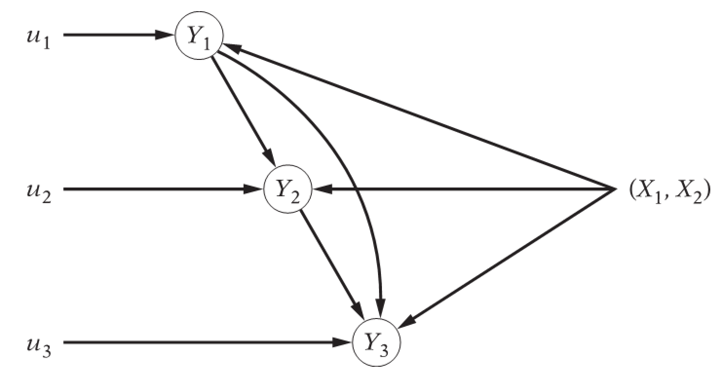
Visualize graphically

We can also visualize it graphically:

wage-price model

Let’s look at the wage-price model:

\[ \begin{cases} \begin{align} P_t &= \beta_0+\beta_1UN_t+\beta_2R_t+\beta_3M_t+u_{t2} &&\text{(price equation)}\\ W_t &= \alpha_0+\alpha_1UN_t+\alpha_2P_t+u_{t1} &&\text{(wage equation)} \end{align} \end{cases} \]

Where:

W, the money wage rate;
UN, unemployment, %;
P, price rate;
R, the cost of capital rate;
M, import price change rate of raw materials.

20.3 Indirect least squares (ILS)

ILS approach with Just Identification model

indirect least squares estimates

For a just or exactly identiﬁed structural equation, the method of obtaining the estimates of the structural coefﬁcients from the OLS estimates of the reduced-form coefﬁcients is known as the method of Indirect Least Squares (ILS), and the estimates thus obtained are known as the indirect least squares estimates.

ILS involves the following three steps:

Step 1. We ﬁrst obtain the reduced-form SEM.
Step 2. We apply OLS to the reduced-form SEM individually.
Step 3. We obtain estimates of the original structural coefﬁcients from the estimated reduced-form coefﬁcients obtained in Step 2. > If an equation is exactly identiﬁed, there is one-to-one mapping between the structural and reduced coefficients.

This operation is permissible since the explanatory variables in these equations are predetermined and hence uncorrelated with the stochastic disturbances. The estimates thus obtained are consistent.对一个恰好识别的结构方程，从约简型系数的OLS估计值获得结构系数估计值的方法叫做间接最小二乘法 (method of indirect least squares, ILS)，而如此得到的估计值称间接最小二乘估计值。间接最小二乘法(ILS方法)包含以下三个步骤:- step 1：先求约简型方程。从结构方程组解出约简型方程，使得在每个方程的因变量都成为唯一的内生变量，并且仅仅是前定变量(外生或滞后内生)和随机误差项的函数。- step 2：对约简型方程逐个应用OLS。因为这些方程中的解释变量是前定的并因而与随机干扰项不相关，所以这种做法是合适的，由此得到的估计值是一致的。- step 3: 从得到的约简型系数的估计值求原始结构系数的估计值。若方程恰可识别，则结构与约简型系数之间有一一对应关系，就是说可以从后者导出前者的唯一估计值。

Case demo: US crop supply and demand

variables

The variables in the US crop supply and demand case are illustrated below

Data set

The data for US crop supply and demand case show here:

Structural SEM

So we can construct the following structural SEM:

\[ \begin{cases} \begin{align} Q &= \alpha_0+\alpha_1P_t+\alpha_2X_t+u_{t1} &(\alpha_1<0,\alpha_2>0) &&\text{(demand function)}\\ Q &= \beta_0+\beta_1P_t+u_{t2} &(\beta_1>0) &&\text{(supply function)} \end{align} \end{cases} \]

where： - \(Q=\)Crop yield index; - \(P=\)Agricultural products purchasing prices index; - \(X=\)Capital personal consumption expenditure.

Reduced SEM

Thus we can obtain the reduced SEM:

\[ \begin{cases} \begin{align} P_t &= \pi_{11}+ \pi_{21}X_t+w_t &&\text{(eq1)}\\ Q_t &= \pi_{12}+\pi_{22}X_t+v_t &&\text{(eq2)} \\ \end{align} \end{cases} \]

and the relationship between structural and reduced coefficients is:

\[ \begin{cases} \begin{align} \pi_{11} &= \frac{\beta_0-\alpha_0}{\alpha_1-\beta_1} \\ \pi_{21} &= - \frac{\alpha_2}{\alpha_1-\beta_1}\\ w_t &= \frac{u_{2t}-u_{t1}}{\alpha_1-\beta_1} \\ \end{align} \end{cases} \]

\[ \begin{cases} \begin{align} \pi_{12} &= \frac{\alpha_1\beta_0-\alpha_0\beta_1}{\alpha_1-\beta_1} \\ \pi_{22} &= - \frac{\alpha_2\beta_1}{\alpha_1-\beta_1} \\ v_t &= \frac{\alpha_1u_{t2}-\beta_1u_{1t}}{\alpha_1-\beta_1} \end{align} \end{cases} \]

Reduced coefficients

For the above reduced SEM, we can use OLS method to obtain the estimated coefficients:

\[ \begin{cases} \begin{align} \widehat{\pi}_{21} &= \frac{\sum{p_t x_t}}{\sum{x^2_t}} &&\text{(slope of the reduced price eq)} \\ \widehat{\pi}_{11} &= \overline{P} - \widehat{\pi}_1 \cdot \overline{X} &&\text{(intercept of the reduced price eq)} \\ \widehat{\pi}_{22} &= \frac{\sum{q_t x_t}}{\sum{x^2_t}} &&\text{(slope of the reduced quantaty eq)} \\ \widehat{\pi}_{12} &= \overline{Q} - \widehat{\pi}_3 \cdot \overline{X} &&\text{(intercept of the reduced quantaty eq)} \end{align} \end{cases} \]

Structural coefficients

Because we already know that the supply equation in the structural SEM is Just identification (please review the order and rank conditions) , hence the structural coefficients of the supply equation can be calculated uniquely with the reduced coefficients.

\[ \begin{cases} \begin{align} \beta_0 &= \pi_{12}+ \beta_1 \pi_{11} \\ \beta_1 &= \frac{\pi_{22}}{\pi_{21}} \\ \end{align} \end{cases} \]

which is:

\[ \begin{cases} \begin{align} \hat{\beta_0} &= \widehat{\pi}_{12}+ \hat{\beta_1} \widehat{\pi}_{11} \\ \hat{\beta_1} &= \frac{\widehat{\pi}_{22}}{\widehat{\pi}_{21}} \\ \end{align} \end{cases} \]

OLS estimates for reduced equation

Next, we carry out OLS regression for the reduced equation.

\[ \begin{cases} \begin{align} P_t &= \pi_{11}+ \pi_{21}X_t+w_t &&\text{(reduced eq1)}\\ Q_t &= \pi_{12}+\pi_{22}X_t+v_t &&\text{(reduced eq2)} \\ \end{align} \end{cases} \]

The regression result of the reduced price equation is:

\[ \begin{alignedat}{999} \begin{split} &\widehat{P}=&&+90.96&&+0.00X_i\\ &(s)&&(4.0517)&&(0.0002)\\ &(t)&&(+22.45)&&(+3.01)\\ &(fit)&&R^2=0.2440&&\bar{R}^2=0.2170\\ &(Ftest)&&F^*=9.04&&p=0.0055 \end{split} \end{alignedat} \]

The regression result of the reduced quantity equation is:

\[ \begin{alignedat}{999} \begin{split} &\widehat{Q}=&&+59.76&&+0.00X_i\\ &(s)&&(1.5600)&&(0.0001)\\ &(t)&&(+38.31)&&(+20.93)\\ &(fit)&&R^2=0.9399&&\bar{R}^2=0.9378\\ &(Ftest)&&F^*=437.95&&p=0.0000 \end{split} \end{alignedat} \]

Obtain structural coefficients

we can obtain the reduced coefficients:

\(\widehat{\pi}_{21}=\) 0.00074
\(\widehat{\pi}_{11}=\) 90.96007

\(\widehat{\pi}_{22}=\) 0.00197
\(\widehat{\pi}_{12}=\) 59.76183

Because supply equation in structural SEM is Just identification, so the structural coefficients of supply equation can be calculated by using the estimated reduced coefficients.

\(\hat{\beta_1} = \frac{\widehat{\pi}_{22}}{\widehat{\pi}_{12}}\) = 0.00197 / 0.00074 = 2.68052 \(\hat{\beta_0} = \widehat{\pi}_{12}+ \hat{\beta_1} \widehat{\pi}_{11}\) = 59.76183 - 2.68052 \(\cdot\) 90.96007 = -184.05874

Therefore, the ILS estimators of supply equation parameters are:

\(\hat{Q_t}=\) -184.05874 + 2.68052 \(P_t\)

Result comparison

As comparison, we will show a “biased” estimation method, which use OLS directly for both quantity and price equation.

Estimation of the supply equation based on the ILS approach: \(\hat{Q_t}=\) -184.05874 + 2.68052 \(P_t\)

Estimation of the supply equation based on the biased OLS approach:

\[ \begin{alignedat}{999} \begin{split} &\widehat{Q}=&&+20.89&&+0.67P_i\\ &(s)&&(23.0396)&&(0.2246)\\ &(t)&&(+0.91)&&(+2.99)\\ &(fit)&&R^2=0.2425&&\bar{R}^2=0.2154\\ &(Ftest)&&F^*=8.96&&p=0.0057 \end{split} \end{alignedat} \]

20.4 Two-stage least square method (2SLS)

2SLS with Overidentification model

Structural SEM

Consider the following structural SEM:

\[ \begin{cases} \begin{alignat}{6} Y_{t1} = & &+ \gamma_{21}Y_{2t} & & +\beta_{01} & + \beta_{11}X_{t1} & + \beta_{21}X_{t2} & +u_{t1} & \text{ (income eq)} \\ Y_{t2} = & + \gamma_{12}Y_{t1} & & & +\beta_{02} & & & + u_{t2} & \text{ (monetary supply eq)} \end{alignat} \end{cases} \]

where: \(Y_1=\) Income; \(Y_2=\) Monetary stock; \(X_1=\) Government expenditure; \(X_2=\) Government spending on goods and services

Using order condition rules and rank condition rules (Review), we can know:

The Income equation is underidentification
if you don’t change the model specification, then god can’t help you!
The monetary supply equation is overidentification it’s easy to prove that if we apply the ILS approach we will obtain two estimates on \(\gamma_{21}\) . Hence it is impossible to determin the exact value.

Instrument variables

Looking for Instrument variables approach to crack the overidentification problems:

In practice, people might want to use OLS to estimate the monetary supply equation, but it will get the biased estimators, because there exist correlationship between \(Y_1\) and \(u_2\) .

Instrument Variable: An agent variable which is highly correlated with \(Y_1\) but have no relationship with \(u_2\) .

if we can find an instrument variable, then we can apply OLS approach directly to estimate the structural monetary supply eqution.

But how does one obtain such an instrumental variable?

One answer is provided by the two-stageleast squares (2SLS), developed independently by Henri Theil and Robert Basmann.

Stage 1 of 2SLS

2SLS method involves two successive applications of OLS. The process is as follows:

Stage 1. To get rid of the likely correlation between \(Y_1\) and \(u_2\) ,apply regresssion \(Y_1\) on all the predetermined variables in the whole system, not just that equation.

\[ \begin{align} Y_{t1} &= \widehat{\pi}_{01} + \widehat{\pi}_{11} X_{t1} + \widehat{\pi}_{21} X_{t2} + \hat{v}_{t1} \\ &= \hat{Y_{t1} } + \hat{v}_{t1} \\ \hat{Y_{t1} }&= \widehat{\pi}_{01} + \widehat{\pi}_{11} X_{t1} + \widehat{\pi}_{21} X_{t2} \end{align} \]

Indicates that the random \(Y_1\) is composed of two parts:

a linear combination of the nonstochastic \(X\)
random component \(\hat{u}_t\)

according to OLS theory, \(\hat {Y}_{t1}\) is not related to \(\hat{v}_{t1}\) (Why?).

Stage 2 of 2SLS

stage 2. Now retransform the overidentification supply equation as follow:

\[ \begin{align} Y_{t2} & = \beta_{02} + \gamma_{12} Y_{t1} + u_{t2} \\ & = \beta_{02} + \gamma_{12} (\hat{Y}_{t1}+\hat{v}_{t1}) + u_{t2} \\ & = \beta_{02} + \gamma_{12} \hat{Y}_{t1}+(\gamma_{12} \hat{v}_{t1} + u_{t2} ) \\ & = \beta_{02} + \gamma_{12} \hat{Y}_{t1}+ u_{t2}^{\ast} \end{align} \]

We can prove that:

the variable \(Y_{t1}\) may be relative with the disturbance term \(u_{t2}\) , which will invalid the OLS approach.
Meanwhile, \(\hat{Y_{1t}}\) is uncorrelated with \(u_{t2}^{\ast}\) asymptotically, that is, in the large sample (or more accurately, as the sample size increases indeﬁnitely).

As a result, OLS can be applied to monetary Eq, which will give consistent estimates of the parameters of the monetary supply function.

2SLS Features (1/4)

Note the following features of 2SLS:

It can be applied to an individual equation in the system without directly taking into account any other equation(s) in the system. Hence, for solving econometric models involving a large number of equations, 2SLS offers an economical method.
Unlike ILS, which provides multiple estimates of parameters in the overidentiﬁed equations, 2SLS provides only one estimate per parameter.
It is easy to apply because all one needs to know is the total number of exogenous or pre-determined variables in the system without knowing any other variables in the system.
Although specially designed to handle overidentiﬁed equations, the method can also be applied to exactly identiﬁed equations. But then ILS and 2SLS will give identical estimates. (Why?)

2SLS Features (2/4)

Note the following features of 2SLS (continue):

If the \(R^2\) values in the reduced-form regressions (that is, Stage 1 regressions) are very high, say, in excess of 0.8, the classical OLS estimates and 2SLS estimates will be very close.

But this result should not be surprising because if the \(R^2\) value in the first stage is very high, it means that the estimated values of the endogenous variables are very close to their actual values.

And hence the latter are less likely to be correlated with the stochastic disturbances in the original structural SEM. (Why?)

2SLS Features (3/4)

Note the following features of 2SLS (continue):

Notice that in reporting the ILS regression we did not state the standard errors of the estimated coefﬁcients . But we can do this for the 2SLS estimates because the structural coefﬁcients are directly estimated from the second-stage (OLS) regressions. > The estimated standard errors in the second-stage regressions need to be modiﬁed because the error term \(u^{\ast}_t\) is, in fact, equal to \(u_{2t}+β_{21}\hat{u}_t\) .

Hence, the variance of \(u^{\ast}_t\) is not exactly equal to the variance of the original \(u_{2t}\) .

2SLS Features (4/4)

Note the following features of 2SLS (continue):

Remarks from Henri Theil:

The statistical justification of the 2SLS is of the large-sample type.

When the equation system contains lagged endogenous variables, the consistency and large-sample normality of the 2SLS coefﬁcient estimators require an additional condition.

Take cautions when lagged endogenous variables are not really predetermined.

Standard error correction: why?

In the regression report of ILS method, we do not give the standard error of the estimated coefficient, but we can give these standard error for the estimator of 2SLS.

Remind \(u^{\ast}_{t2}=u_{t2}+\gamma_{12}\hat{v}_{t1}\)
It will imply \(u^{\ast}_{t2} \neq u_{t2}\) , and then we need to calculate the “correct” standard error for the purpose of inference.

For the specific method of error correction, please refer to appendix 20a.2 of the textbook (Damodar Gujarati).

In the following cases illurtration, we will show the 2SLS estimates without error correction and the 2SLS estimates with error correction respectively.

Standard error correction: focus stage 2

The process for error correction show as below.

stage 2: The regression form of the supply equation is

\[ \begin{align} Y_{t2} & = \beta_{02} + \gamma_{12} Y_{1t} + u_{2t} \\ & = \beta_{02} + \gamma_{12} (\hat{Y_{1t}}+\hat{v}_{t1}) + u_{2t} \\ & = \beta_{02} + \gamma_{12} \hat{Y_{1t}}+(\gamma_{12} \hat{v}_{t1} + u_{t2} ) \\ & = \beta_{02} + \gamma_{12} \hat{Y_{1t}}+ u_{t2}^{\ast} \end{align} \]

Where:

\(u^{\ast}_{t2}=u_{t2}+\gamma_{12}\hat{v}_{t1}\)

Standard error correction: focus stage 2

stage 2: the estimation for the parameter \(\gamma_{12}\) is \(\hat{\gamma}_{12}\), and its standard error \(s.e_{\hat{\gamma}_{12}}\) can be calculated as below.

\[ \begin{align} Y_{t2} & = \beta_{02} + \gamma_{12} \hat{Y_{1t}}+ u_{t2}^{\ast} \end{align} \]

\[ \begin{align} s.e_{\hat{\gamma}_{21}} & = \frac{\hat{\sigma}^2_{u^{\ast}_{t2}}}{\sum{\hat{y}^2_{t1}}}\\ \hat{\sigma}^2_{u^{\ast}_{t2}} & =\frac{ \sum{\left ( u^{\ast}_{t2} \right )^2} }{n-2} = \frac{ \sum{\left (Y_{t2}-\hat{\beta}_{02} -\hat{\gamma}_{12}\hat{Y}_{1t} \right )^2} }{n-2} \end{align} \]

Standard error correction: results

In fact, we know \(u^{\ast}_{t2} \neq u_{t2}\) , which means \(\hat{\sigma}_{u^{\ast}_{t2}} \neq \hat{\sigma}_{u_{t2}}\) .
Thus we can obtain \(\hat{\sigma}_{u_{t2}}\) .

\[ \begin{align} \hat{u}_{t2} &= Y_{t2} - \hat{\beta}_{02} - \hat{\gamma}_{12}Y_{t1} \\ \hat{\sigma}^2_{u_{2t}} & =\frac{ \sum{\left ( u_{2t} \right )^2} }{n-2} = \frac{ \sum{\left (Y_{t2}-\hat{\beta}_{02} -\hat{\gamma}_{12}Y_{1t} \right )^2} }{n-2} \end{align} \]

Standard error correction: for coefficients

Therefore, in order to correct the standard error of the coefficients estimated by stage 2 regression, it is necessary to multiply the standard error of each coefficient by the following error correction factor.

\[ \begin{align} \eta &= \frac{ \hat{\sigma}^2_{u_{t2}} } {\hat{\sigma}^2_{u^{\ast}_{t2}} } \end{align} \]

\[ \begin{align} s.e^{\ast}_{\hat{\gamma}_{12}} & = s.e_{\hat{\gamma}_{12}} \cdot \eta = s.e_{\hat{\gamma}_{12}} \cdot \frac{ \hat{\sigma}^2_{u_{t2}} } {\hat{\sigma}^2_{u^{\ast}_{t2}} } \\ s.e^{\ast}_{\hat{\beta}_{02}} & = s.e_{\hat{\beta}_{02}} \cdot \eta = s.e_{\hat{\beta}_{20}} \cdot \frac{ \hat{\sigma}^2_{u_{t2}} } {\hat{\sigma}^2_{u^{\ast}_{t2}} } \end{align} \]

Case study and application for 2SLS approach

variable description

data set

Modeling scenario 1 and 2SLS without error correction

Only the money supply equation is overidentifiable

Structural SEM and identification problems

Therefore, we can construct the following structural SEM:

\[ \begin{cases} \begin{alignat}{6} Y_{t1} = \beta_{01} & &+ \gamma_{21}Y_{t2} & & + \beta_{11}X_{t1} & + \beta_{21}X_{t2} & & +u_{t1} && \text{ (income eq)} \\ Y_{t2} = \beta_{02} & + \gamma_{12}Y_{1t} & & & & & & + u_{t2} && \text{ (money supply eq)} \end{alignat} \end{cases} \]

Where:

\(Y_1=GDP\) (gross domestic product GDP);
\(Y_2=M2\) (money supply);
\(X_1=GDPI\) (Private domestic investment);
\(X_2=FEDEXP\) (Federal expenditure)

Stage 1 of 2SLS: fit the reduced equation 1

\[ \begin{cases} \begin{alignat}{6} Y_{t1} &&= \beta_{01} && &&+ \gamma_{21}Y_{t2} && + \beta_{11}X_{t1} && + \beta_{21}X_{t2} && +u_{t1} && \text{ (income eq)} \\ Y_{t2} &&= \beta_{02} && + \gamma_{12}Y_{1t} && && && && + u_{t2} && \text{ (money supply eq)} \end{alignat} \end{cases} \]

stage 1: Estimate the regression of \(Y_1\) to all predetermined variables in the structural SEM (not only in the equation under consideration), and obtain \(\hat{Y}_{t1}; \hat {n} _ {t1}\) .

That is:

\[ \begin{align} Y_{1t} &= \widehat{\pi_0} + \widehat{\pi_1} X_{1t} + \widehat{\pi_2} X_{2t} + \hat{v}_{t1} \\ &= \hat{Y_{1t} } + \hat{v}_{t1} \end{align} \]

Regression results of stage 1:

\[ \begin{alignedat}{999} \begin{split} &\widehat{Y1}=&&+2689.85&&+1.87X1_i&&+2.03X2_i\\ &(s)&&(67.9874)&&(0.1717)&&(0.1075)\\ &(t)&&(+39.56)&&(+10.89)&&(+18.93)\\ &(fit)&&R^2=0.9964&&\bar{R}^2=0.9962 &&\\ &(Ftest)&&F^*=4534.36&&p=0.0000 && \end{split} \end{alignedat} \]

stage 1 of 2SLS: fitted \(\hat{Y}_1\) and \(\hat{v}_1\)

At the same time, we can obtain \(\hat{Y }_{t1} ;\hat{v}_{t1}\) :

Stage 2 of 2SLS: result of estimation for \(Y_2\)

stage 2: Now transform the overidentification supply equation as follows:

\[ \begin{align} Y_{t2} & = \beta_{02} + \gamma_{12} \hat{Y}_{1t}+ u_{t2}^{\ast} \end{align} \]

Using the new variables in stage 1 results, and apply OLS estimation to obtain:

\[ \begin{alignedat}{999} \begin{split} &\widehat{Y2}=&&-2440.20&&+0.79Y1.hat_i\\ &(s)&&(127.3738)&&(0.0178)\\ &(t)&&(-19.16)&&(+44.52)\\ &(fit)&&R^2=0.9831&&\bar{R}^2=0.9826\\ &(Ftest)&&F^*=1982.40&&p=0.0000 \end{split} \end{alignedat} \]

Comparison (1/2): OLS approach directly

As comparison, we give a “biased” estimation with OLS method directly to the money supply equation, and obtain following result:

\[ \begin{alignedat}{999} \begin{split} &\widehat{Y2}=&&-2430.34&&+0.79Y1_i\\ &(s)&&(127.2148)&&(0.0178)\\ &(t)&&(-19.10)&&(+44.51)\\ &(fit)&&R^2=0.9831&&\bar{R}^2=0.9826\\ &(Ftest)&&F^*=1980.77&&p=0.0000 \end{split} \end{alignedat} \]

Comparison (2/2): Raw R report

The R raw report for the biased regression show as:


Call:
lm(formula = models_money$mod.ols, data = us_money_new)

Residuals:
   Min     1Q Median     3Q    Max 
-418.3 -151.7   40.2  143.5  380.8 

Coefficients:
              Estimate Std. Error t value Pr(>|t|)    
(Intercept) -2.430e+03  1.272e+02  -19.10   <2e-16 ***
Y1           7.905e-01  1.776e-02   44.51   <2e-16 ***
---
Signif. codes:  0 '***' 0.001 '**' 0.01 '*' 0.05 '.' 0.1 ' ' 1

Residual standard error: 229.1 on 34 degrees of freedom
Multiple R-squared:  0.9831,    Adjusted R-squared:  0.9826 
F-statistic:  1981 on 1 and 34 DF,  p-value: < 2.2e-16

Modeling scenario 2

both income equation and money supply equation are over-identifiable

Improved structural SEM and identification problems

Different from the former structural SEM, we can construct the improved one:

\[ \begin{cases} \begin{alignat}{6} Y_{t1} = \beta_{01} & &+ \gamma_{12}Y_{t2} & & + \beta_{11}X_{t1} & + \beta_{21}X_{t2} & & & +u_{t1} & \text{ (income eq)} \\ Y_{t2} = \beta_{02} & + \gamma_{12}Y_{1t} & & & & &+ \beta_{12}Y_{1,t-1} &+ \beta_{22}Y_{2,t-1} & + u_{t2} & \text{ (money supply eq)} \end{alignat} \end{cases} \]

Next, we judge the identification problem according to order condition rules 2 :

The number of predetermineed variables in the structural SEM is \(K=5\) .
The first equation: the number of predetermined variables is \(k=3\) , and \((K-k)=2\) . Also the number of endogenous variables is \(m=2\) , and \((m-1)=1\) . We will see \((K-k)>(m-1)\) . So the first equation is overidentification.
The second equation: the number of predetermined variables is \(k=3\) , and \((K-k)=2\) ; Also the number of endogenous variables is \(m=2\) , and \((m-1)=1\) . We will see \((K-k)>(m-1)\) . Thus it is also overidentification.

Stage 1 of 2SLS: reduced equation 1 and 2

Now, we will use two-stage least squares (2SLS) to get consistent estimates for both income equation and money supply equation.

Stage 1:

Estimate the regression of \(Y_1\) to all predetermined variables in the structural SEM (not only in the equation under consideration), and obtain \(\hat{Y}_{t1} ;\hat{v}^{\ast}_{t1}\) .
Meanwhile, estimate the regression of \(Y_2\) to all predetermined variables in the structural SEM (not only in the equation under consideration), and obtain \(\hat{Y}_{t2} ;\hat{v}^{\ast}_{t2}\) ：

\[ \begin{align} Y_{t1} &= \widehat{\pi}_{01} + \widehat{\pi}_{11} X_{t1} + \widehat{\pi}_{21} X_{t2} + \widehat{\pi}_{31} Y_{t-1,1} + \widehat{\pi}_{41} Y_{t-1,2}+ \hat{v}_{t1} \\ &= \hat{Y}_{1t} +\hat{v}_{t1} \\ Y_{t2} &= \widehat{\pi}_{02} + \widehat{\pi}_{12} X_{t1} + \widehat{\pi}_{22} X_{t2} + \widehat{\pi}_{32} Y_{t-1,1} + \widehat{\pi}_{42} Y_{t-1,2}+ \hat{v}_{t2} \\ &= \hat{Y}_{t2} +\hat{v}_{t2} \end{align} \]

Stage 1 of 2SLS: fit the reduced equation 1

OLS regression results of new income equation at stage 1:

\[ \begin{alignedat}{999} \begin{split} &\widehat{Y1}=&&+1098.90&&+0.98X1_i&&+0.77X2_i\\ &(s)&&(185.5566)&&(0.1308)&&(0.1831)\\ &(t)&&(+5.92)&&(+7.50)&&(+4.19)\\ &(cont.)&&+0.59Y1.l1_i&&-0.01Y2.l1_i &&\\ &(s)&&(0.0667)&&(0.0721) &&\\ &(t)&&(+8.87)&&(-0.10) &&\\ &(fit)&&R^2=0.9990&&\bar{R}^2=0.9989 &&\\ &(Ftest)&&F^*=7857.58&&p=0.0000 && \end{split} \end{alignedat} \]

Stage 1 of 2SLS: fit the reduced equation 2

OLS regression results of new money supply equation at stage 1:

\[ \begin{alignedat}{999} \begin{split} &\widehat{Y2}=&&-207.14&&+0.20X1_i&&-0.35X2_i\\ &(s)&&(184.9121)&&(0.1303)&&(0.1824)\\ &(t)&&(-1.12)&&(+1.53)&&(-1.95)\\ &(cont.)&&+0.06Y1.l1_i&&+1.06Y2.l1_i &&\\ &(s)&&(0.0665)&&(0.0718) &&\\ &(t)&&(+0.94)&&(+14.78) &&\\ &(fit)&&R^2=0.9985&&\bar{R}^2=0.9983 &&\\ &(Ftest)&&F^*=5050.57&&p=0.0000 && \end{split} \end{alignedat} \]

Stage 1 of 2SLS: fitted \(\hat{Y}_i\) and \(\hat{v}_i\)

Hence, we can obtain new variables from the two former regressions results respectively: \(\hat{Y}_{t1} ;\hat{v}_{t1}\) , and \(\hat{Y}_{t2} ;\hat{v}_{t2}\) .

Stage 2 of 2SLS: estimate the structural equation 1 and 2

Stage 2:

The re-transformed new income equation and the money supply equation are:

\[ \begin{align} Y_{t1} &= \beta_{01} + \gamma_{21} \hat{Y}_{t2} + \beta_{11}X_{t1} + \beta_{21}X_{t2} +u^{\ast}_{t1} \\ Y_{t2} &= \beta_{20} + \gamma_{12} \hat{Y}_{1t} + \beta_{12}Y_{t-1,1} + \beta_{22}Y_{t-1,2} + u^{\ast}_{t2} \end{align} \]

And then, we can conduct these new equations by using the former variables frome stage 1.

Stage 2 of 2SLS: OLS estimation for the new income equation

OLS estimation results of new income equation in stage 2:

\[ \begin{alignedat}{999} \begin{split} &\widehat{Y1}=&&+2723.68&&+0.22Y2.hat_i&&+1.71X1_i\\ &(s)&&(67.5331)&&(0.1156)&&(0.1848)\\ &(t)&&(+40.33)&&(+1.90)&&(+9.27)\\ &(cont.)&&+1.57X2_i && &&\\ &(s)&&(0.2623) && &&\\ &(t)&&(+5.98) && &&\\ &(fit)&&R^2=0.9966&&\bar{R}^2=0.9963 &&\\ &(Ftest)&&F^*=3073.97&&p=0.0000 && \end{split} \end{alignedat} \]

Stage 2 of 2SLS: OLS estimation for the new money supply equation

OLS estimation results of the new money supply equation in stage 2:

\[ \begin{alignedat}{999} \begin{split} &\widehat{Y2}=&&-228.13&&+0.11Y1.hat_i&&-0.03Y1.l1_i\\ &(s)&&(153.6925)&&(0.1431)&&(0.1481)\\ &(t)&&(-1.48)&&(+0.77)&&(-0.17)\\ &(cont.)&&+0.93Y2.l1_i && &&\\ &(s)&&(0.0618) && &&\\ &(t)&&(+15.10) && &&\\ &(fit)&&R^2=0.9981&&\bar{R}^2=0.9979 &&\\ &(Ftest)&&F^*=5461.60&&p=0.0000 && \end{split} \end{alignedat} \]

Stage 2 of 2SLS: Raw R report for the new income equation

The R raw report of OLS estimation for the new income equation in stage 2:


Call:
lm(formula = models_money2$mod2.stage2.1, data = us_money_new2)

Residuals:
    Min      1Q  Median      3Q     Max 
-360.45  -66.79   35.70   81.22  186.18 

Coefficients:
             Estimate Std. Error t value Pr(>|t|)    
(Intercept) 2723.6809    67.5331  40.331  < 2e-16 ***
Y2.hat         0.2192     0.1156   1.896   0.0673 .  
X1             1.7142     0.1848   9.275 1.87e-10 ***
X2             1.5690     0.2623   5.981 1.29e-06 ***
---
Signif. codes:  0 '***' 0.001 '**' 0.01 '*' 0.05 '.' 0.1 ' ' 1

Residual standard error: 130.1 on 31 degrees of freedom
  (1 observation deleted due to missingness)
Multiple R-squared:  0.9966,    Adjusted R-squared:  0.9963 
F-statistic:  3074 on 3 and 31 DF,  p-value: < 2.2e-16

Stage 2 of 2SLS: Raw R report for the new money supply equation

The R raw report of OLS estimation for the new money supply equation in stage 2:


Call:
lm(formula = models_money2$mod2.stage2.1, data = us_money_new2)

Residuals:
    Min      1Q  Median      3Q     Max 
-360.45  -66.79   35.70   81.22  186.18 

Coefficients:
             Estimate Std. Error t value Pr(>|t|)    
(Intercept) 2723.6809    67.5331  40.331  < 2e-16 ***
Y2.hat         0.2192     0.1156   1.896   0.0673 .  
X1             1.7142     0.1848   9.275 1.87e-10 ***
X2             1.5690     0.2623   5.981 1.29e-06 ***
---
Signif. codes:  0 '***' 0.001 '**' 0.01 '*' 0.05 '.' 0.1 ' ' 1

Residual standard error: 130.1 on 31 degrees of freedom
  (1 observation deleted due to missingness)
Multiple R-squared:  0.9966,    Adjusted R-squared:  0.9963 
F-statistic:  3074 on 3 and 31 DF,  p-value: < 2.2e-16

Simultaneous 2SLS approach with error correction automatically (tidy report)

By using R systemfit package, we can apply the two-stage least square method with “error correction”, and the report summarized as follows:

Simultaneous 2SLS approach with error correction automatically (raw report)

By using R systemfit package, we can apply the two-stage least square method with “error correction”, and the detail report show as follows:


systemfit results 
method: 2SLS 

        N DF    SSR   detRCov   OLS-R2 McElroy-R2
system 70 62 749260 107381032 0.997082   0.998059

     N DF    SSR      MSE     RMSE       R2   Adj R2
eq1 35 31 549669 17731.24 133.1587 0.996492 0.996153
eq2 35 31 199592  6438.44  80.2399 0.998006 0.997813

The covariance matrix of the residuals
         eq1      eq2
eq1 17731.24 -2603.96
eq2 -2603.96  6438.44

The correlations of the residuals
         eq1      eq2
eq1  1.00000 -0.24371
eq2 -0.24371  1.00000


2SLS estimates for 'eq1' (equation 1)
Model Formula: Y1 ~ Y2 + X1 + X2
Instruments: ~X1 + X2 + Y1.l1 + Y2.l1

               Estimate  Std. Error  t value   Pr(>|t|)    
(Intercept) 2723.680944   69.101729 39.41553 < 2.22e-16 ***
Y2             0.219243    0.118317  1.85302    0.07342 .  
X1             1.714216    0.189119  9.06422 3.1717e-10 ***
X2             1.569039    0.268427  5.84531 1.9068e-06 ***
---
Signif. codes:  0 '***' 0.001 '**' 0.01 '*' 0.05 '.' 0.1 ' ' 1

Residual standard error: 133.158716 on 31 degrees of freedom
Number of observations: 35 Degrees of Freedom: 31 
SSR: 549668.549447 MSE: 17731.243531 Root MSE: 133.158716 
Multiple R-Squared: 0.996492 Adjusted R-Squared: 0.996153 


2SLS estimates for 'eq2' (equation 2)
Model Formula: Y2 ~ Y1 + Y1.l1 + Y2.l1
Instruments: ~X1 + X2 + Y1.l1 + Y2.l1

                Estimate   Std. Error  t value   Pr(>|t|)    
(Intercept) -228.1320387  157.9454624 -1.44437    0.15867    
Y1             0.1099682    0.1470504  0.74783    0.46020    
Y1.l1         -0.0250416    0.1522272 -0.16450    0.87040    
Y2.l1          0.9329562    0.0635111 14.68965 1.7764e-15 ***
---
Signif. codes:  0 '***' 0.001 '**' 0.01 '*' 0.05 '.' 0.1 ' ' 1

Residual standard error: 80.239917 on 31 degrees of freedom
Number of observations: 35 Degrees of Freedom: 31 
SSR: 199591.774884 MSE: 6438.444351 Root MSE: 80.239917 
Multiple R-Squared: 0.998006 Adjusted R-Squared: 0.997813

Comparison to OLS approach directly (biased estimation)

“biased” OLS estimation results of the income equation:

\[ \begin{alignedat}{999} \begin{split} &\widehat{Y1}=&&+2706.39&&+0.17Y2_i&&+1.75X1_i\\ &(s)&&(67.6150)&&(0.1115)&&(0.1864)\\ &(t)&&(+40.03)&&(+1.51)&&(+9.39)\\ &(cont.)&&+1.68X2_i && &&\\ &(s)&&(0.2552) && &&\\ &(t)&&(+6.60) && &&\\ &(fit)&&R^2=0.9966&&\bar{R}^2=0.9963 &&\\ &(Ftest)&&F^*=3139.86&&p=0.0000 && \end{split} \end{alignedat} \]

“biased” OLS estimates of the money supply equation:

\[ \begin{alignedat}{999} \begin{split} &\widehat{Y2}=&&-206.53&&-0.02Y1_i&&+0.10Y1.l1_i\\ &(s)&&(154.4428)&&(0.1178)&&(0.1252)\\ &(t)&&(-1.34)&&(-0.14)&&(+0.79)\\ &(cont.)&&+0.94Y2.l1_i && &&\\ &(s)&&(0.0622) && &&\\ &(t)&&(+15.14) && &&\\ &(fit)&&R^2=0.9981&&\bar{R}^2=0.9979 &&\\ &(Ftest)&&F^*=5362.58&&p=0.0000 && \end{split} \end{alignedat} \]

20.5 Truffle supply and demand

Case of Truffle supply and demand

Variables description

Data set

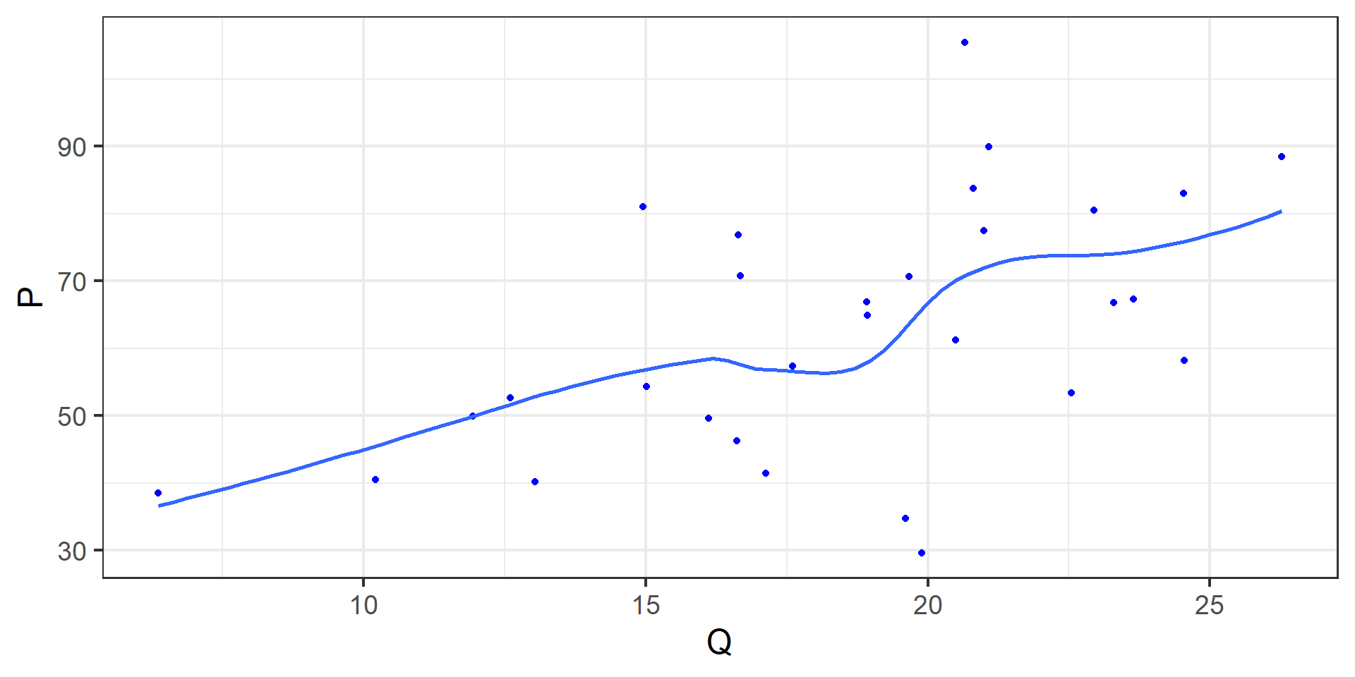
Scatter

The scatter plot on truffle quantity Q and truffle market price P is given below:

The structural SEM

Given the structural SEM:

\[ \begin{cases} \begin{align} Q_i &= \alpha_0+\alpha_1P_i+\alpha_2PS_i+\alpha_3DI_i+u_{i1} &&\text{(demand function)}\\ Q_i &= \beta_0+\beta_1P_i+\beta_2PF_i+u_{i2} &&\text{(supply function)} \end{align} \end{cases} \]

The reduced SEM

We can get the reduced SEM:

\[ \begin{cases} \begin{align} P_i &= \pi_{01}+ \pi_{11}PS_i+\pi_{21}DI_i+\pi_{31}PF_i+v_{t1}\\ Q_i &= \pi_{02}+\pi_{12}PS_t+\pi_{22}DI_i+\pi_{32}PF_i+v_{t2} \end{align} \end{cases} \]

Also we obtain the relationship between structural and reduced coefficients:

\[ \begin{cases} \begin{align} & \pi_{01} = \frac{\beta_0-\alpha_0}{\alpha_1-\beta_1} \\ & \pi_{11} = - \frac{\alpha_2}{\alpha_1-\beta_1} \\ & \pi_{21} = - \frac{\alpha_3}{\alpha_1-\beta_1} \\ & \pi_{31} = \frac{\beta_2}{\alpha_1-\beta_1} \\ & v_{t1} = \frac{u_{2t}-u_{1t}}{\alpha_1-\beta_1} && \end{align} \end{cases} \]

\[ \begin{cases} \begin{align} & \pi_{02} = - \frac{\alpha_1\beta_0-\alpha_0\beta_1}{\alpha_1-\beta_1} \\ & \pi_{12} = - \frac{\alpha_2\beta_1}{\alpha_1-\beta_1} \\ & \pi_{22} = - \frac{\alpha_3\beta_1}{\alpha_1-\beta_1} \\ & \pi_{32} = \frac{\alpha_1\beta_2}{\alpha_1-\beta_1} \\ & v_{t2} = \frac{\alpha_1u_{2t}-\beta_1u_{1t}}{\alpha_1-\beta_1} \end{align} \end{cases} \]

Simple OLS solution: stylized report

We can apply OLS method directly. Of course estimation results will be biased.

stylized results of bias OLS estimation for the demand equation:

\[ \begin{alignedat}{999} \begin{split} &\widehat{Q}=&&+1.09&&+0.02P_i&&+0.71PS_i\\ &(s)&&(3.7116)&&(0.0768)&&(0.2143)\\ &(t)&&(+0.29)&&(+0.30)&&(+3.31)\\ &(cont.)&&+0.08DI_i && &&\\ &(s)&&(1.1909) && &&\\ &(t)&&(+0.06) && &&\\ &(fit)&&R^2=0.4957&&\bar{R}^2=0.4375 &&\\ &(Ftest)&&F^*=8.52&&p=0.0004 && \end{split} \end{alignedat} \]

stylized results of bias OLS estimation for the supply equation:

\[ \begin{alignedat}{999} \begin{split} &\widehat{Q}=&&+20.03&&+0.34P_i&&-1.00PF_i\\ &(s)&&(1.2220)&&(0.0217)&&(0.0764)\\ &(t)&&(+16.39)&&(+15.54)&&(-13.10)\\ &(fit)&&R^2=0.9019&&\bar{R}^2=0.8946 &&\\ &(Ftest)&&F^*=124.08&&p=0.0000 && \end{split} \end{alignedat} \]

Simple OLS solution: R code (`lm`)

# set equation systems
eq.D <-formula( Q~P + PS + DI)
eq.S <-formula( Q~P + PF)

# fit using direct `OLS` method
ols.D <- lm(formula = eq.D, data = truffles)
ols.S <- lm(formula = eq.S, data = truffles)
# estimation summary
smry.olsD <- summary(ols.D)
smry.olsS <- summary(ols.S)

Simple OLS solution: R report for demand eqation


Call:
lm(formula = eq.D, data = truffles)

Residuals:
   Min     1Q Median     3Q    Max 
-7.155 -1.936 -0.374  2.396  6.335 

Coefficients:
            Estimate Std. Error t value Pr(>|t|)   
(Intercept)  1.09105    3.71158   0.294  0.77112   
P            0.02330    0.07684   0.303  0.76418   
PS           0.71004    0.21432   3.313  0.00272 **
DI           0.07644    1.19086   0.064  0.94931   
---
Signif. codes:  0 '***' 0.001 '**' 0.01 '*' 0.05 '.' 0.1 ' ' 1

Residual standard error: 3.46 on 26 degrees of freedom
Multiple R-squared:  0.4957,    Adjusted R-squared:  0.4375 
F-statistic:  8.52 on 3 and 26 DF,  p-value: 0.0004159

Simple OLS solution: R report for supply eqation


Call:
lm(formula = eq.S, data = truffles)

Residuals:
    Min      1Q  Median      3Q     Max 
-3.7830 -0.8530  0.2270  0.7579  3.3475 

Coefficients:
            Estimate Std. Error t value Pr(>|t|)    
(Intercept) 20.03278    1.22197   16.39 1.47e-15 ***
P            0.33799    0.02174   15.54 5.42e-15 ***
PF          -1.00092    0.07639  -13.10 3.23e-13 ***
---
Signif. codes:  0 '***' 0.001 '**' 0.01 '*' 0.05 '.' 0.1 ' ' 1

Residual standard error: 1.498 on 27 degrees of freedom
Multiple R-squared:  0.9019,    Adjusted R-squared:  0.8946 
F-statistic: 124.1 on 2 and 27 DF,  p-value: 2.448e-14

Simultaneous OLS solution: R code (`symtemfit`)

# load pkg
require(systemfit)
# set equation systems
eq.D <- Q~P + PS + DI
eq.S <- Q~P + PF
eq.sys <- list(eq.D, eq.S)
# system fit using `OLS` method
system.ols <- systemfit(
  formula = eq.sys,
  method = "OLS",
  data = truffles
)
# estimation summary
smry.ols <- summary(system.ols)

Simultaneous OLS solution: R report (`symtemfit`)


systemfit results 
method: OLS 

        N DF     SSR detRCov   OLS-R2 McElroy-R2
system 60 53 371.764 23.5756 0.698799   0.808917

     N DF      SSR      MSE    RMSE       R2   Adj R2
eq1 30 26 311.2096 11.96960 3.45971 0.495720 0.437534
eq2 30 27  60.5546  2.24276 1.49758 0.901878 0.894610

The covariance matrix of the residuals
         eq1     eq2
eq1 11.96960 1.80814
eq2  1.80814 2.24276

The correlations of the residuals
        eq1     eq2
eq1 1.00000 0.34898
eq2 0.34898 1.00000


OLS estimates for 'eq1' (equation 1)
Model Formula: Q ~ P + PS + DI

             Estimate Std. Error t value  Pr(>|t|)   
(Intercept) 1.0910453  3.7115804 0.29396 0.7711247   
P           0.0232954  0.0768423 0.30316 0.7641812   
PS          0.7100395  0.2143246 3.31292 0.0027193 **
DI          0.0764442  1.1908551 0.06419 0.9493078   
---
Signif. codes:  0 '***' 0.001 '**' 0.01 '*' 0.05 '.' 0.1 ' ' 1

Residual standard error: 3.459711 on 26 degrees of freedom
Number of observations: 30 Degrees of Freedom: 26 
SSR: 311.209627 MSE: 11.969601 Root MSE: 3.459711 
Multiple R-Squared: 0.49572 Adjusted R-Squared: 0.437534 


OLS estimates for 'eq2' (equation 2)
Model Formula: Q ~ P + PF

              Estimate Std. Error  t value   Pr(>|t|)    
(Intercept) 20.0327764  1.2219720  16.3938 1.3323e-15 ***
P            0.3379875  0.0217445  15.5435 5.3291e-15 ***
PF          -1.0009246  0.0763902 -13.1028 3.2352e-13 ***
---
Signif. codes:  0 '***' 0.001 '**' 0.01 '*' 0.05 '.' 0.1 ' ' 1

Residual standard error: 1.497585 on 27 degrees of freedom
Number of observations: 30 Degrees of Freedom: 27 
SSR: 60.554565 MSE: 2.242762 Root MSE: 1.497585 
Multiple R-Squared: 0.901878 Adjusted R-Squared: 0.89461

IV 2SLS solution: R code (`symtemfit`)

# load pkg
require(systemfit)
# set equation systems
eq.D <- Q~P + PS + DI
eq.S <- Q~P + PF
eq.sys <- list(eq.D, eq.S)
# set instruments
instr <- ~ PS + DI + PF
# system fit using `2SLS` method
system.iv <- systemfit(
  formula = eq.sys, inst = instr,
  method = "2SLS",
  data = truffles
)
# estimation summary
smry.iv <- summary(system.iv)

IV-2SLS Solution: R report (`symtemfit`)


systemfit results 
method: 2SLS 

        N DF     SSR detRCov   OLS-R2 McElroy-R2
system 60 53 692.472 49.8028 0.438964   0.807408

     N DF      SSR      MSE    RMSE        R2    Adj R2
eq1 30 26 631.9171 24.30450 4.92996 -0.023950 -0.142098
eq2 30 27  60.5546  2.24276 1.49758  0.901878  0.894610

The covariance matrix of the residuals
         eq1     eq2
eq1 24.30451 2.16943
eq2  2.16943 2.24276

The correlations of the residuals
        eq1     eq2
eq1 1.00000 0.29384
eq2 0.29384 1.00000


2SLS estimates for 'eq1' (equation 1)
Model Formula: Q ~ P + PS + DI
Instruments: ~PS + DI + PF

             Estimate Std. Error  t value  Pr(>|t|)   
(Intercept) -4.279471   5.543884 -0.77193 0.4471180   
P           -0.374459   0.164752 -2.27287 0.0315350 * 
PS           1.296033   0.355193  3.64881 0.0011601 **
DI           5.013977   2.283556  2.19569 0.0372352 * 
---
Signif. codes:  0 '***' 0.001 '**' 0.01 '*' 0.05 '.' 0.1 ' ' 1

Residual standard error: 4.92996 on 26 degrees of freedom
Number of observations: 30 Degrees of Freedom: 26 
SSR: 631.917143 MSE: 24.304505 Root MSE: 4.92996 
Multiple R-Squared: -0.02395 Adjusted R-Squared: -0.142098 


2SLS estimates for 'eq2' (equation 2)
Model Formula: Q ~ P + PF
Instruments: ~PS + DI + PF

              Estimate Std. Error  t value   Pr(>|t|)    
(Intercept) 20.0328022  1.2231148  16.3785 1.5543e-15 ***
P            0.3379816  0.0249196  13.5629 1.4344e-13 ***
PF          -1.0009094  0.0825279 -12.1281 1.9456e-12 ***
---
Signif. codes:  0 '***' 0.001 '**' 0.01 '*' 0.05 '.' 0.1 ' ' 1

Residual standard error: 1.497585 on 27 degrees of freedom
Number of observations: 30 Degrees of Freedom: 27 
SSR: 60.554565 MSE: 2.242762 Root MSE: 1.497585 
Multiple R-Squared: 0.901878 Adjusted R-Squared: 0.89461

IV-2SLS Solution: tidy report (`symtemfit`)

Comparison (1/2): results of the reduced equations by OLS directly

The OLS regression results of reduced price equation:

\[ \begin{alignedat}{999} \begin{split} &\widehat{P}=&&-32.51&&+1.71PS_i&&+7.60DI_i\\ &(s)&&(7.9842)&&(0.3509)&&(1.7243)\\ &(t)&&(-4.07)&&(+4.87)&&(+4.41)\\ &(cont.)&&+1.35PF_i && &&\\ &(s)&&(0.2985) && &&\\ &(t)&&(+4.54) && &&\\ &(fit)&&R^2=0.8887&&\bar{R}^2=0.8758 &&\\ &(Ftest)&&F^*=69.19&&p=0.0000 && \end{split} \end{alignedat} \]

The OLS regression results of reduced quantity equation:

\[ \begin{alignedat}{999} \begin{split} &\widehat{Q}=&&+7.90&&+0.66PS_i&&+2.17DI_i\\ &(s)&&(3.2434)&&(0.1425)&&(0.7005)\\ &(t)&&(+2.43)&&(+4.61)&&(+3.09)\\ &(cont.)&&-0.51PF_i && &&\\ &(s)&&(0.1213) && &&\\ &(t)&&(-4.18) && &&\\ &(fit)&&R^2=0.6974&&\bar{R}^2=0.6625 &&\\ &(Ftest)&&F^*=19.97&&p=0.0000 && \end{split} \end{alignedat} \]

Comparison (2/2): results of the structural equations by OLS directly

We can apply OLS method directly. Of course estimation results will be biased.

tidy results of bias OLS estimation for the demand equation:

tidy results of bias OLS estimation for the supply equation:

20.6 Cod supply and demand

Cod supply and demand

Variables description

Sample data set

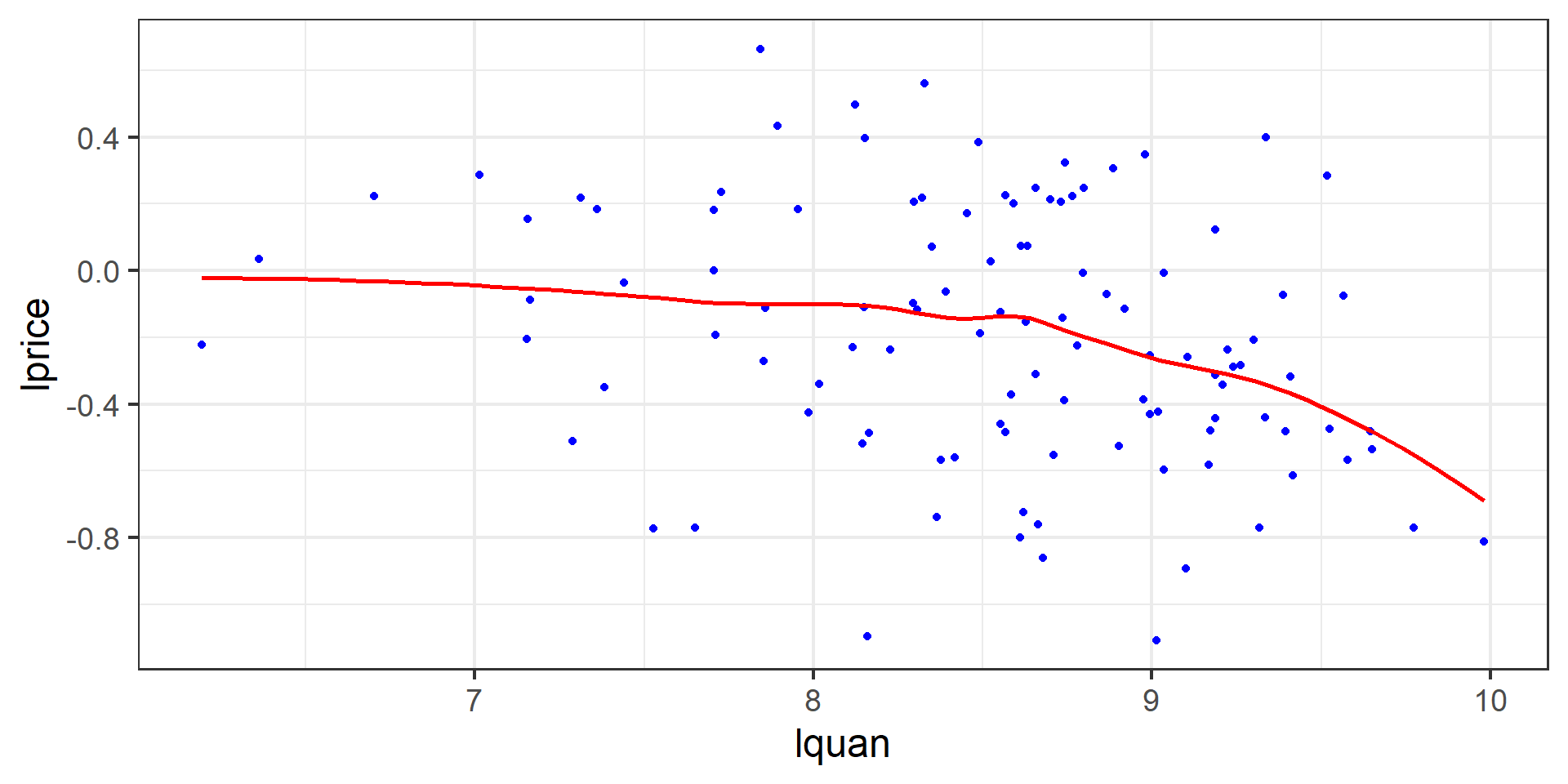
Scatter

The structural and reduced SEM

Given the structural SEM:

\[ \begin{cases} \begin{align} lquan_t &= \alpha_0+\alpha_1lprice_t+\alpha_2mon_t+\alpha_3tue_t+\alpha_4wen_t+\alpha_5thu_t+u_{1t} &&\text{(demand eq)}\\ lquan_t &= \beta_0+\beta_1lprice_t+\beta_3stormy_t+u_{2t} &&\text{(supply eq)} \end{align} \end{cases} \]

We can obtain the reduced SEM:

\[ \begin{cases} \begin{align} lquan_t &= \pi_0 + \pi_1mon_t+\pi_2tue_t+\pi_3wen_t+\pi_4thu_t +\pi_5stormy_t+v_t &&\text{(reduced eq1)}\\ lprice_t &= \pi_0 + \pi_1mon_t+\pi_2tue_t+\pi_3wen_t+\pi_4thu_t +\pi_5stormy_t+v_t &&\text{(reduced eq2)}\\ \end{align} \end{cases} \]

OLS regression results of the reduced SEM

The regression results of reduced quantity equation show as follows:

\[ \begin{alignedat}{999} &\widehat{lquan}=&&+8.81&&+0.10mon&&-0.48tue&&-0.55wed&&+0.05thu&&-0.39stormy\\ &\text{(t)}&&(59.9225)&&(0.4891)&&(-2.4097)&&(-2.6875)&&(0.2671)&&(-2.6979)\\ &\text{(se)}&&(0.1470)&&(0.2065)&&(0.2011)&&(0.2058)&&(0.2010)&&(0.1437)\\ &\text{(fitness)}&& n=111;&& R^2=0.1934;&& \bar{R^2}=0.1550\\ & && F^{\ast}=5.03;&& p=0.0004\\ \end{alignedat} \]

The regression results of reduced price equation show as follows:

\[ \begin{alignedat}{999} &\widehat{lprice}=&&-0.27&&-0.11mon&&-0.04tue&&-0.01wed&&+0.05thu&&+0.35stormy\\ &\text{(t)}&&(-3.5569)&&(-1.0525)&&(-0.3937)&&(-0.1106)&&(0.4753)&&(4.6387)\\ &\text{(se)}&&(0.0764)&&(0.1073)&&(0.1045)&&(0.1069)&&(0.1045)&&(0.0747)\\ &\text{(fitness)}&& n=111;&& R^2=0.1789;&& \bar{R^2}=0.1398\\ & && F^{\ast}=4.58;&& p=0.0008 \end{alignedat} \]

IV-2SLS regression results: R code

# set equation systems
fish.D <- formula(lquan ~ lprice + mon + tue + wed + thu)
fish.S <- formula(lprice ~ lquan + stormy)
fish.eqs <- list(fish.D, fish.S)
# set instruments
fish.ivs <- ~ mon + tue + wed + thu + stormy
# system fit using `2SLS` method
fish.sys <- systemfit(fish.eqs,
  method = "2SLS",
  inst = fish.ivs, data = fultonfish
)
# estimation summary
fish.smry <- summary(fish.sys)

IV-2SLS regression results: raw report


systemfit results 
method: 2SLS 

         N  DF    SSR  detRCov   OLS-R2 McElroy-R2
system 222 213 65.577 0.055061 0.143396   0.308369

      N  DF     SSR      MSE     RMSE       R2   Adj R2
eq1 111 105 52.0903 0.496098 0.704342 0.139124 0.098130
eq2 111 108 13.4867 0.124877 0.353379 0.159506 0.143941

The covariance matrix of the residuals
          eq1       eq2
eq1 0.4960983 0.0830042
eq2 0.0830042 0.1248767

The correlations of the residuals
         eq1      eq2
eq1 1.000000 0.333484
eq2 0.333484 1.000000


2SLS estimates for 'eq1' (equation 1)
Model Formula: lquan ~ lprice + mon + tue + wed + thu
Instruments: ~mon + tue + wed + thu + stormy

              Estimate Std. Error  t value   Pr(>|t|)    
(Intercept)  8.5059113  0.1661669 51.18896 < 2.22e-16 ***
lprice      -1.1194169  0.4286450 -2.61152  0.0103334 *  
mon         -0.0254022  0.2147742 -0.11827  0.9060766    
tue         -0.5307694  0.2080001 -2.55177  0.0121574 *  
wed         -0.5663511  0.2127549 -2.66199  0.0089895 ** 
thu          0.1092673  0.2087866  0.52334  0.6018373    
---
Signif. codes:  0 '***' 0.001 '**' 0.01 '*' 0.05 '.' 0.1 ' ' 1

Residual standard error: 0.704342 on 105 degrees of freedom
Number of observations: 111 Degrees of Freedom: 105 
SSR: 52.090321 MSE: 0.496098 Root MSE: 0.704342 
Multiple R-Squared: 0.139124 Adjusted R-Squared: 0.09813 


2SLS estimates for 'eq2' (equation 2)
Model Formula: lprice ~ lquan + stormy
Instruments: ~mon + tue + wed + thu + stormy

                Estimate   Std. Error  t value   Pr(>|t|)    
(Intercept) -2.90660e-01  1.03438e+00 -0.28100 0.77924840    
lquan        3.78095e-05  1.19797e-01  0.00032 0.99974876    
stormy       3.35276e-01  8.58664e-02  3.90463 0.00016468 ***
---
Signif. codes:  0 '***' 0.001 '**' 0.01 '*' 0.05 '.' 0.1 ' ' 1

Residual standard error: 0.353379 on 108 degrees of freedom
Number of observations: 111 Degrees of Freedom: 108 
SSR: 13.486684 MSE: 0.124877 Root MSE: 0.353379 
Multiple R-Squared: 0.159506 Adjusted R-Squared: 0.143941

IV-2SLS regression results: tidy report

Comparison with the biased OLS estimation: R code

# demand equation
fish.D <- formula(lquan ~ lprice + mon + tue + wed + thu)
ols_fish_D <- lm(fish.D, data = fultonfish)

# supply equation
fish.S <- formula(lprice ~ lquan + stormy)
ols_fish_S <- lm(fish.S, data = fultonfish)

Comparison with the biased OLS estimation: raw report

raw R summry of bias OLS estimation for the demand equation:


Call:
lm(formula = fish.D, data = fultonfish)

Residuals:
     Min       1Q   Median       3Q      Max 
-2.23844 -0.36737  0.08832  0.42304  1.24866 

Coefficients:
            Estimate Std. Error t value Pr(>|t|)    
(Intercept)  8.60689    0.14304  60.170  < 2e-16 ***
lprice      -0.56255    0.16821  -3.344  0.00114 ** 
mon          0.01432    0.20265   0.071  0.94381    
tue         -0.51624    0.19769  -2.611  0.01034 *  
wed         -0.55537    0.20232  -2.745  0.00712 ** 
thu          0.08162    0.19782   0.413  0.68073    
---
Signif. codes:  0 '***' 0.001 '**' 0.01 '*' 0.05 '.' 0.1 ' ' 1

Residual standard error: 0.6702 on 105 degrees of freedom
Multiple R-squared:  0.2205,    Adjusted R-squared:  0.1834 
F-statistic:  5.94 on 5 and 105 DF,  p-value: 7.08e-05

Comparison with the biased OLS estimation: stylized results

tidy results of bias OLS estimation for the demand equation:

\[ \begin{alignedat}{999} \begin{split} &\widehat{lquan}=&&+8.61&&-0.56lprice_i&&+0.01mon_i\\ &(s)&&(0.1430)&&(0.1682)&&(0.2026)\\ &(t)&&(+60.17)&&(-3.34)&&(+0.07)\\ &(cont.)&&-0.52tue_i&&-0.56wed_i&&+0.08thu_i\\ &(s)&&(0.1977)&&(0.2023)&&(0.1978)\\ &(t)&&(-2.61)&&(-2.75)&&(+0.41)\\ &(fit)&&R^2=0.2205&&\bar{R}^2=0.1834 &&\\ &(Ftest)&&F^*=5.94&&p=0.0001 && \end{split} \end{alignedat} \]

tidy results of bias OLS estimation for the supply equation:

\[ \begin{alignedat}{999} \begin{split} &\widehat{lprice}=&&+0.60&&-0.10lquan_i&&+0.30stormy_i\\ &(s)&&(0.3948)&&(0.0455)&&(0.0742)\\ &(t)&&(+1.51)&&(-2.26)&&(+4.01)\\ &(fit)&&R^2=0.1974&&\bar{R}^2=0.1825 &&\\ &(Ftest)&&F^*=13.28&&p=0.0000 && \end{split} \end{alignedat} \]

Comparison: the biased OLS estimation

raw R summry of bias OLS estimation for the supply equation:


Call:
lm(formula = fish.S, data = fultonfish)

Residuals:
     Min       1Q   Median       3Q      Max 
-0.89381 -0.21934  0.00898  0.20711  0.82067 

Coefficients:
            Estimate Std. Error t value Pr(>|t|)    
(Intercept)  0.59605    0.39481   1.510  0.13404    
lquan       -0.10273    0.04554  -2.256  0.02608 *  
stormy       0.29798    0.07422   4.015  0.00011 ***
---
Signif. codes:  0 '***' 0.001 '**' 0.01 '*' 0.05 '.' 0.1 ' ' 1

Residual standard error: 0.3453 on 108 degrees of freedom
Multiple R-squared:  0.1974,    Adjusted R-squared:  0.1825 
F-statistic: 13.28 on 2 and 108 DF,  p-value: 6.985e-06

20.7 Exercise and computation

Labor market of married Working Women

Story background

Let’s consider the labor market for married women already in the workforce.

We will use the data on working, married women in wooldridge::mroz to estimate the labor supply and wage demand equations by 2SLS.

The full set of instruments includes educ, age, kidslt6, nwifeinc, exper, and exper2.

Variables and definition

We will focus on the following variables.

lwage: log(wage)
hours: hours worked, 1975
kidslt6: kids less than 6 years
age: woman’s age in yrs
educ: years of schooling
exper: actual labor mkt exper
expersq: exper^2
nwifeinc: (faminc - wage*hours)/1000

SEM setting: the structrual equations

\[ \begin{aligned} \text { hours } & =\alpha_1 \log ( wage)+\beta_{10}+\beta_{11} { educ }+\beta_{12} age+\beta_{13} { kidslt6 } &&\\ &+\beta_{14} { nwifeinc }+u_1 &&\text{(supply)}\\ \log ({ wage }) &=\alpha_2 { hours }+\beta_{20}+\beta_{21} { educ }+\beta_{22} { exper } +\beta_{23} { exper }^2+ u_2 && \quad \text{(demand)} \end{aligned} \]

In the demand function, we write the wage offer as a function of hours and the usual productivity variables.
All variables except hours and log(wage) are assumed to be exogenous.
educ might be correlated with omitted ability in either equation. Here, we just ignore the omitted ability problem.

SEM setting: the reduced equations

\[ \begin{alignedat}{8} \text { hours } & =\pi_{10}+\pi_{11} { educ }+\pi_{12} age+\pi_{13} { kidslt6 } +\pi_{14} { nwifeinc }\\ &+\pi_{15} { exper } +\pi_{16} {exper}^2 +v_1 \\ \log ({ wage }) &=\pi_{20}+\pi_{21} { educ }+\pi_{22} age+\pi_{23} { kidslt6 } +\pi_{24} { nwifeinc } \\ &+\pi_{25} { exper } +\pi_{26} {exper}^2+ v_2 \end{alignedat} \]

Exercise tasks 1/2: system fit with TSLS


systemfit results 
method: 2SLS 

         N  DF       SSR detRCov   OLS-R2 McElroy-R2
system 856 845 773893318  155089 -2.00762   0.748802

      N  DF         SSR         MSE        RMSE        R2    Adj R2
eq1 428 423 1.95266e+02 4.61621e-01    0.679427  0.125654  0.117385
eq2 428 422 7.73893e+08 1.83387e+06 1354.204549 -2.007617 -2.043253

The covariance matrix of the residuals
            eq1         eq2
eq1    0.461621    -831.543
eq2 -831.542683 1833869.960

The correlations of the residuals
          eq1       eq2
eq1  1.000000 -0.903769
eq2 -0.903769  1.000000


2SLS estimates for 'eq1' (equation 1)
Model Formula: lwage ~ hours + educ + exper + expersq
Instruments: ~age + kidslt6 + nwifeinc + educ + exper + expersq

                Estimate   Std. Error  t value   Pr(>|t|)    
(Intercept) -0.655725423  0.337788290 -1.94123   0.052894 .  
hours        0.000125900  0.000254611  0.49448   0.621223    
educ         0.110330004  0.015524358  7.10690 5.0768e-12 ***
exper        0.034582356  0.019491555  1.77422   0.076746 .  
expersq     -0.000705769  0.000454080 -1.55428   0.120865    
---
Signif. codes:  0 '***' 0.001 '**' 0.01 '*' 0.05 '.' 0.1 ' ' 1

Residual standard error: 0.679427 on 423 degrees of freedom
Number of observations: 428 Degrees of Freedom: 423 
SSR: 195.265558 MSE: 0.461621 Root MSE: 0.679427 
Multiple R-Squared: 0.125654 Adjusted R-Squared: 0.117385 


2SLS estimates for 'eq2' (equation 2)
Model Formula: hours ~ lwage + educ + age + kidslt6 + nwifeinc
Instruments: ~age + kidslt6 + nwifeinc + educ + exper + expersq

              Estimate Std. Error  t value   Pr(>|t|)    
(Intercept) 2225.66187  574.56413  3.87365 0.00012424 ***
lwage       1639.55563  470.57569  3.48415 0.00054535 ***
educ        -183.75128   59.09981 -3.10917 0.00200323 ** 
age           -7.80609    9.37801 -0.83238 0.40566400    
kidslt6     -198.15431  182.92914 -1.08323 0.27932494    
nwifeinc     -10.16959    6.61474 -1.53741 0.12494168    
---
Signif. codes:  0 '***' 0.001 '**' 0.01 '*' 0.05 '.' 0.1 ' ' 1

Residual standard error: 1354.204549 on 422 degrees of freedom
Number of observations: 428 Degrees of Freedom: 422 
SSR: 773893123.12815 MSE: 1833869.960019 Root MSE: 1354.204549 
Multiple R-Squared: -2.007617 Adjusted R-Squared: -2.043253

Exercise tasks 2/2: OLS estimator and several tests

So we should conduct OLS estimation and several tests as we have learned.

Conduct OLS estimation directly for each structural equation.
Weak instrument test (Restricted F test or Cragg-donald test).
Instrument Exogeneity test (J-test).
Regressor Endogeneity test (Wu-Hausman test).

Find these results and get the conclusion!