Advanced Econometrics III
(Econometrics III)
Chapter 19. What is the Identification Problem ?
Hu Huaping (胡华平)
huhuaping01 at hotmail.com
School of Economics and Management (经济管理学院)
2026-05-30
Part 2:Simultaneous Equation Models (SEM)
Chapter 17. Endogeneity and Instrumental Variables
Chapter 18. Why Should We Concern SEM ?
Chapter 19. What is the Identification Problem ?
Chapter 20. How to Estimate SEM ?
Chapter 19. What is the Identification Problem ?
19.1 Identification Problem
Identification problem of SEM
The identification problem means whether numerical estimates of the structural parameters can be obtained from the estimated reduced coefficients.
Identification status:
If the estimator of structural parameter can be obtained, the equation is said to be Identified, and there may be two district situations:
Just/Exact Identification: The unique estimator of the structure parameter can be obtained.
Overidentification: More than one estimator of a structural parameter can be obtained.
If the estimator of structural parameter cannot be obtained, the particular equation is said to be Underidentification.
Example
The structural SEM
Consider the following SEM for supply and demand:
\[ \begin{cases} \begin{align} Q &= \alpha_0+\alpha_1P_t+u_{t1} &(\alpha_1<0) &&\text{(demand function)}\\ Q &= \beta_0+\beta_1P_t+u_{t2} &(\beta_1>0) &&\text{(supply function)} \end{align} \end{cases} \]
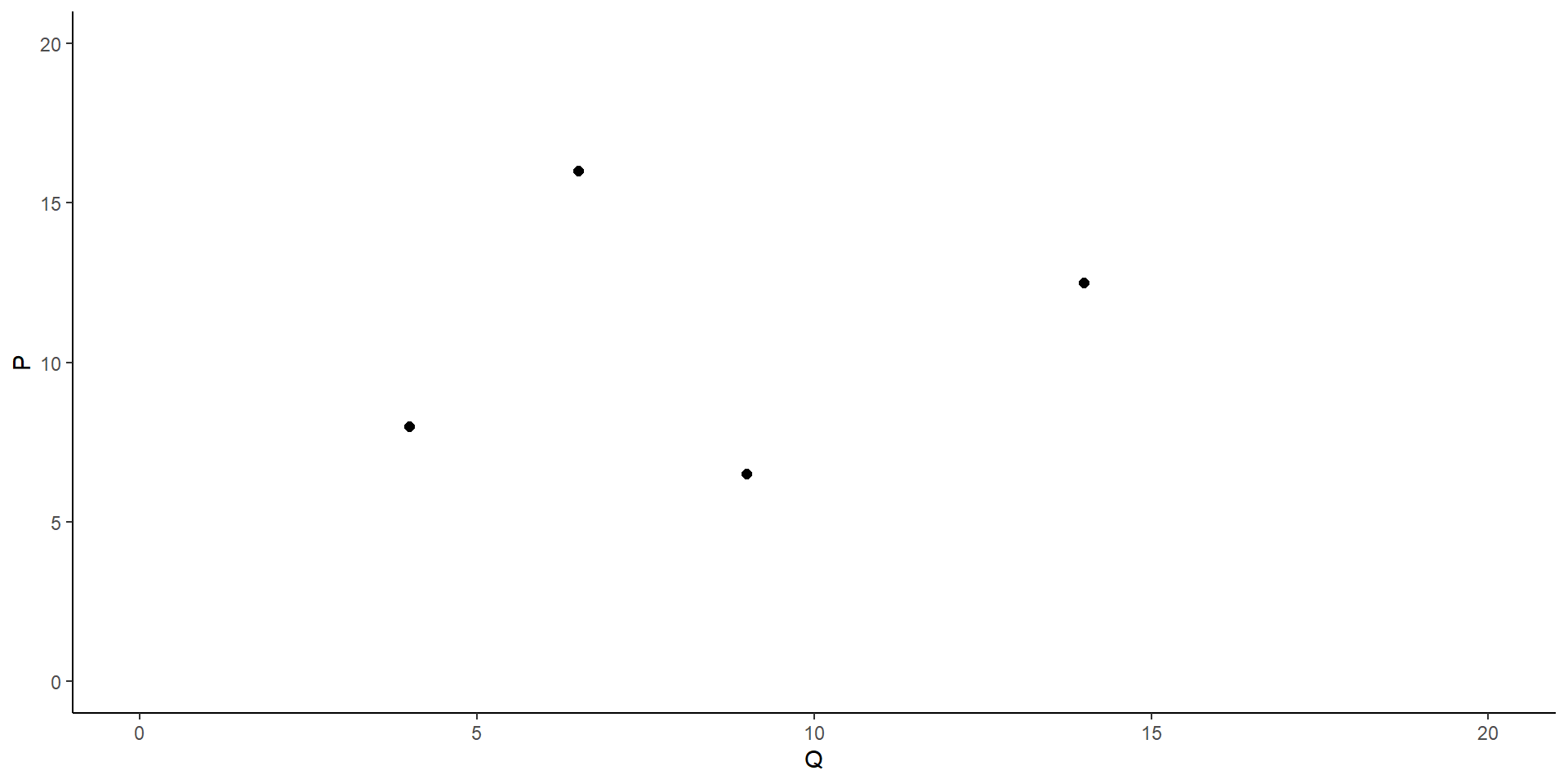
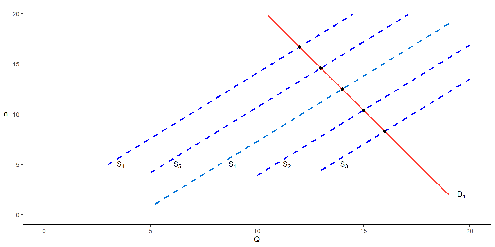
Scatter plots
Equilibrium point of supply and demand
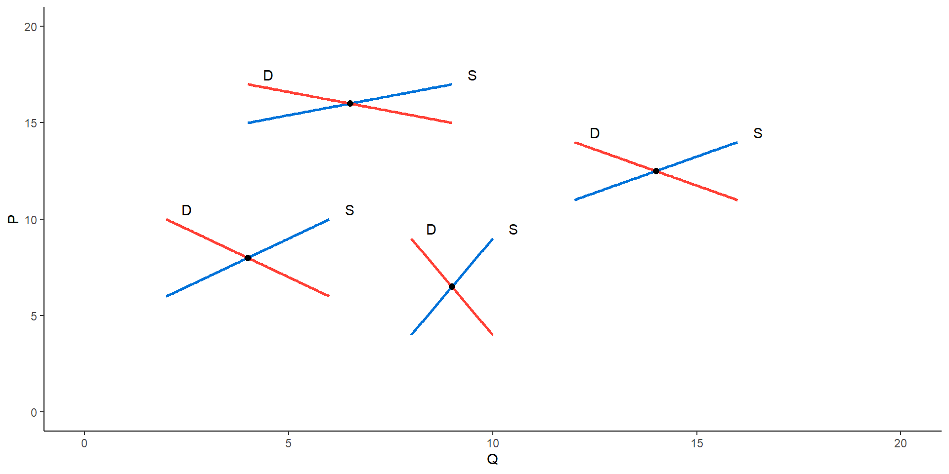
Underidentification
We can’t be sure which of the entire family of supply and demand curves is responsible for this point. thus the supply and demand equation are both underidentification.
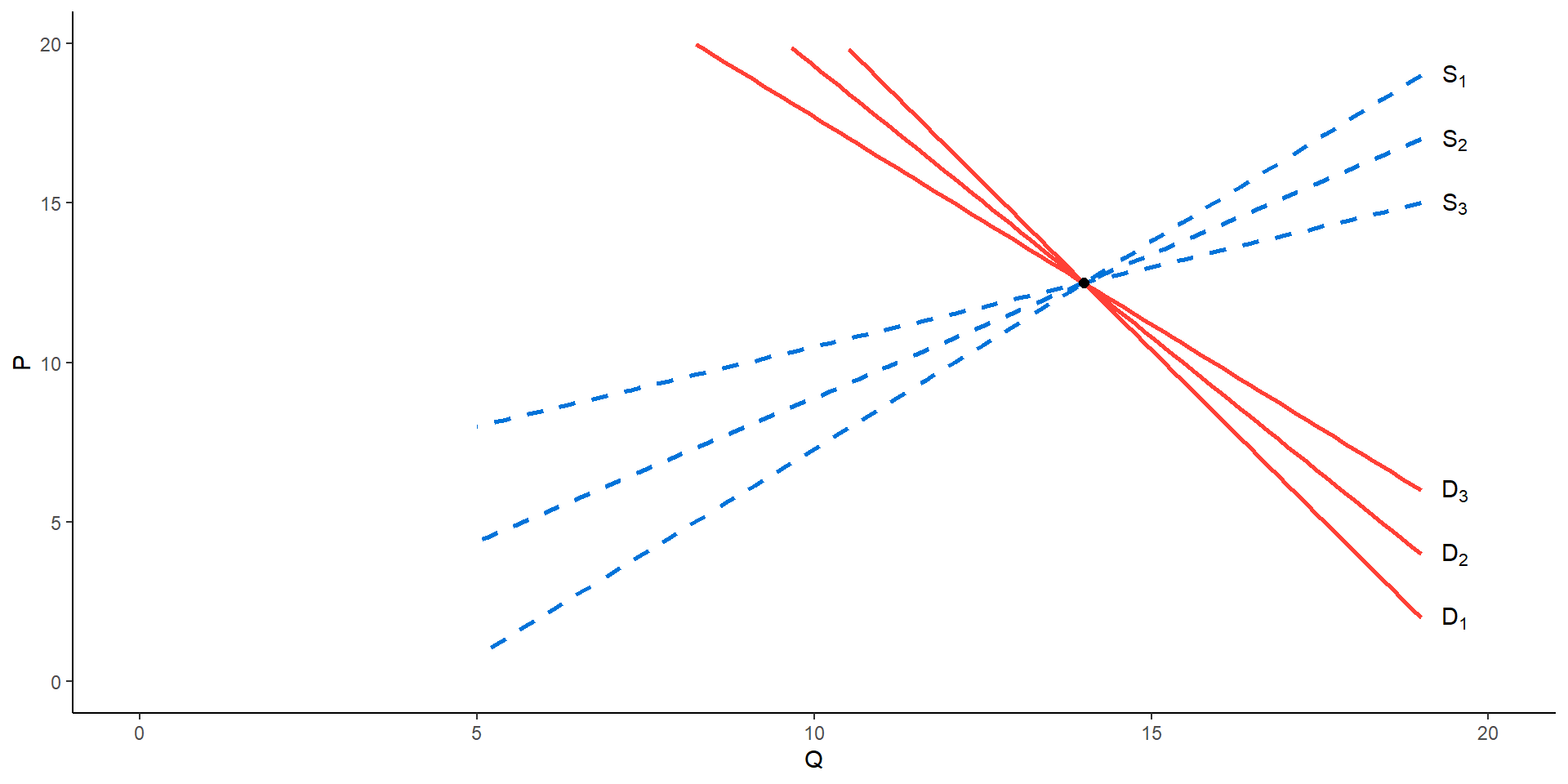
The supply curve can be identified
If the demand curve shifts over time due to changes in income, tastes, etc., and the supply curve remains relatively stable, the scatter will show a Supply Curve. In this case, we say that the supply curve is Exact Identification.
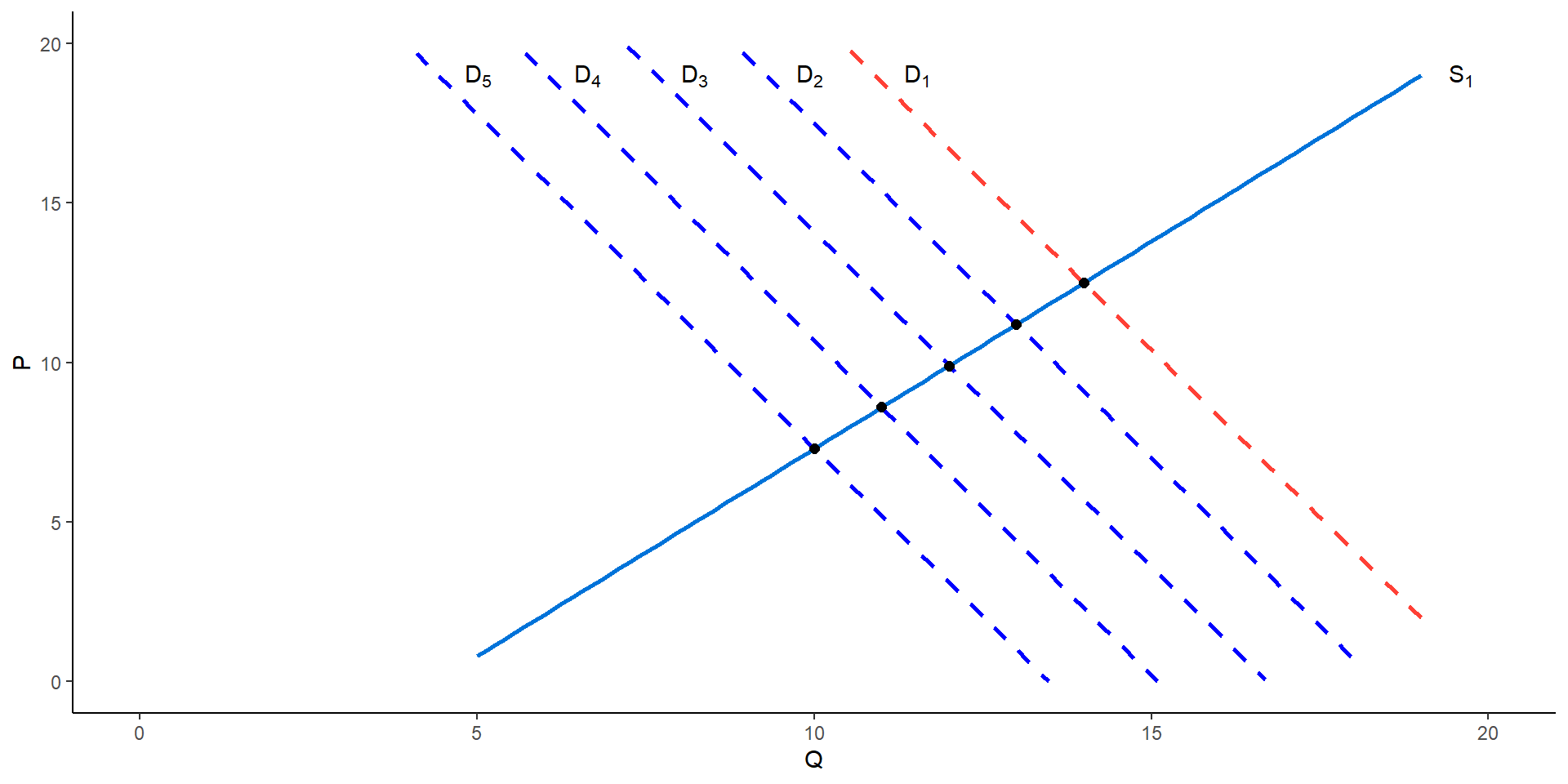
The demand curve can be identified
If the supply curve shifs over time due to changes in climatic conditions or other external factors, but the demand curve remains relatively stable, the scatter will show a demand curve. In this case, we say that the demand curve is identified.
Under identification
Structural and reduced SEM
Give the Structural SEM:
\[ \begin{cases} \begin{align} Q_t &= \alpha_0+\alpha_1P_t+u_{t1} &(\alpha_1<0) &&\text{(demand function)}\\ Q_t &= \beta_0+\beta_1P_t+u_{t2} &(\beta_1>0) &&\text{(supply function)}\\ \end{align} \end{cases} \]
It’s easy to obtain the Reduced SEM:
\[ \begin{cases} \begin{align} P_t &= \pi_{11} +v_{t1} \\ Q_t &= \pi_{12} +v_{t2} \end{align} \end{cases} \]
Obviously, the structural SEM is underidentification! (Why?)
number of structural parameters? 2
number of reduced parameters? 0
An made-up “hybrid” equation
\[ \begin{cases} \begin{align} \lambda Q &= \lambda\alpha_0+\lambda\alpha_1P_t+\lambda u_{t1} &(\alpha_1<0) \text{(transformation 1)}\\ (1-\lambda)Q &= (1-\lambda)\beta_0+(1-\lambda)\beta_1P_t+(1-\lambda)u_{t2} &(\beta_1>0) \text{(transformation 2)} \end{align} \end{cases} \]
Further, we can construct the following “hybrid” equation:
\[ \begin{align} Q_t &= \lambda\alpha_0+(1-\lambda)\beta_0 +(\lambda\alpha_1+(1-\lambda)\beta_1 )P_t+ \lambda u_{1t}+(1-\lambda)u_{t2} & \text{(hybrid equation)} \\ \end{align} \]
And denoted as:
\[ \begin{align} Q_t &= \gamma_0 +\gamma_1P_t+w_t \\ \end{align} \]
Where:
\[ \begin{cases} \begin{align} \gamma_0 & = \lambda\alpha_0+(1-\lambda)\beta_0 \\ \gamma_1 &= \lambda\alpha_1+(1-\lambda)\beta_1 \\ w_t &= \lambda u_{1t}+(1-\lambda)u_{t2} \end{align} \end{cases} \]
This hybrid equation is indistinguishable from any of the structural equations!
So the original structural SEM is underidentification!
Just identification
Structural and reduced SEM
Given Structural SEM ( \(I=\) income of the consumer):
\[ \begin{cases} \begin{align} Q_t &= \alpha_0+\alpha_1P_t+\alpha_2I_t+u_{t1} &(\alpha_1<0,\alpha_2>0) &&\text{(demand function)}\\ Q_t &= \beta_0+\beta_1P_t+u_{t2} &(\beta_1>0) &&\text{(supply function)} \end{align} \end{cases} \]
We can obtain the Reduced SEM:
\[ \begin{cases} \begin{align} P_t &= \pi_{11}+ \pi_{21}I_t+v_{t1} \\ Q_t &= \pi_{12}+ \pi_{22}I_t+v_{t2}\\ \end{align} \end{cases} \]
\[ \begin{cases} \begin{alignedat}{3} & \pi_{11} = \frac{\beta_0-\alpha_0}{\alpha_1-\beta_1}; \quad & \pi_{21} = - \frac{\alpha_2}{\alpha_1-\beta_1} ; \quad & v_{t1} = \frac{u_{t2}-u_{t1}}{\alpha_1-\beta_1} \\ & \pi_{12} = \frac{\alpha_1\beta_0-\alpha_0\beta_1}{\alpha_1-\beta_1};\quad & \pi_{22} = - \frac{\alpha_2\beta_1}{\alpha_1-\beta_1} ;\quad & v_{t2} = \frac{\alpha_1u_{t2}-\beta_1u_{t1}}{\alpha_1-\beta_1} \end{alignedat} \end{cases} \]
Part equation just-identified
Question:
Can the aforementioned structural equation be identified?
- number of reduced parameters?
- number of structural parameters?
Answer:
Only 4 reduced parameters: \(\pi_{11},\pi_{21},\pi_{12},\pi_{22}\)
But 5 structural parameters: \(\alpha_0,\alpha_1,\alpha_2,\beta_0,\beta_1\)
Therefore, it is impossible to completely solve all 5 structural parameters.
However, the supply equation is Exact identification, because:
\[ \begin{align} \beta_0 = \pi_{12}-\beta_1\pi_{11} ; \quad \beta_1 = \frac{\pi_{22}}{\pi_{21}} \end{align} \]
But there is no unique way of estimating the parameters of the demand function.
Therefore, the demand equation remains underidentified.
Structural SEM
Given Structural SEM ( \(P_{t-1}=\) price lagged one period):
\[ \begin{cases} \begin{align} Q_t &= \alpha_0+\alpha_1P_t+\alpha_2I_t+u_{t1} &(\alpha_1<0,\alpha_2>0) &&\text{(demand function)}\\ Q_t &= \beta_0+\beta_1P_t+ \beta_2P_{t-1}+u_{t2} &(\beta_1>0,\beta_2>0) &&\text{(supply function)} \end{align} \end{cases} \]
where the demand function remains as before but the supply function includes an additional explanatory variable, price lagged one period.
Reduced SEM
We can obtain the Reduced SEM:
\[ \begin{cases} \begin{align} P_t &= \pi_{11}+ \pi_{21}I_t + \pi_{31}P_{t-1} +v_{t1} \\ Q_t &= \pi_{12}+ \pi_{22}I_t + \pi_{32}P_{t-1} +v_{t2}\\ \end{align} \end{cases} \]
And obtain the relationship between the structural coefficients and the reduced coefficients.
\[ \begin{cases} \begin{alignedat}{3} & \pi_{11} = \frac{\beta_0-\alpha_0}{\alpha_1-\beta_1}; \quad & \pi_{21} = - \frac{\alpha_2}{\alpha_1-\beta_1} ; \quad & \pi_{31} = - \frac{\beta_2}{\alpha_1-\beta_1} ; \quad & v_{t1} = \frac{u_{t2}-u_{t1}}{\alpha_1-\beta_1} \\ & \pi_{12} = \frac{\alpha_1\beta_0-\alpha_0\beta_1}{\alpha_1-\beta_1};\quad & \pi_{22} = - \frac{\alpha_2\beta_1}{\alpha_1-\beta_1} ;\quad & \pi_{32} = \frac{\alpha_1\beta_2}{\alpha_1-\beta_1} ;\quad & v_{t2} = \frac{\alpha_1u_{t2}-\beta_1u_{t1}}{\alpha_1-\beta_1} \end{alignedat} \end{cases} \]
So, can we calculate the unique structural coefficients by using the numerical reduced coefficients?
All equations just-identified
Question:
Can the aforementioned structural equation be identified?
number of reduced parameters?
number of structural parameters?
Answer:
there are 6 reduced parameters: \(\pi_{11},\pi_{21},\pi_{31};\pi_{12},\pi_{22},\pi_{32}\)
and 6 structural parameters: \(\alpha_0,\alpha_1,\alpha_2;\beta_0,\beta_1,\beta_2\)
Therefore, the parameters of both the SEM equations can be identified, and the system as a whole can be identified exactly.
Over-identification
Structural SEM
Now suppose we consider the following structural SEM for demand-and-supply:
\[ \begin{cases} \begin{align} Q_t &= \alpha_0+\alpha_1P_t+\alpha_2I_t+\alpha_3R_t+u_{t1} &(\alpha_1<0,\alpha_2>0) &&\text{(demand function)}\\ Q_t &= \beta_0+\beta_1P_t+\beta_2P_{t-1}+u_{t2} &(\beta_1,\beta_2>0) &&\text{(supply function)} \end{align} \end{cases} \]
Where the supply function remains as before but the demand function includes two additional explanatory variables, income( \(I_{t}\) ) and wealth( \(R_t\) ).
Questions:Can you transform the structural SEM to get the reduced SEM?
Reduced SEM
We can get the reduced SEM and the relationship between Structural and reduced pars:
\[ \begin{cases} \begin{align} P_t &= \pi_{11}+ \pi_{21}I_t+\pi_{31}R_t+\pi_{41}P_{t-1}+v_{t1} \\ Q_t &= \pi_{12}+\pi_{22}I_t+\pi_{32}R_t+\pi_{42}P_{t-1}+v_{t2} \end{align} \end{cases} \]
\[ \begin{cases} \begin{align} & \pi_{11} = \frac{\beta_0-\alpha_0}{\alpha_1-\beta_1} \\ & \pi_{21} = - \frac{\alpha_2}{\alpha_1-\beta_1} \\ & \pi_{31} = - \frac{\alpha_3}{\alpha_1-\beta_1} \\ & \pi_{41} = \frac{\beta_2}{\alpha_1-\beta_1} \\ & v_{t1} = \frac{u_{t2}-u_{t1}}{\alpha_1-\beta_1} \end{align} \end{cases} \]
\[ \begin{cases} \begin{align} & \pi_{12} = - \frac{\alpha_1\beta_0-\alpha_0\beta_1}{\alpha_1-\beta_1} \\ & \pi_{22} = - \frac{\alpha_2\beta_1}{\alpha_1-\beta_1} \\ & \pi_{32} = - \frac{\alpha_3\beta_1}{\alpha_1-\beta_1} \\ & \pi_{42} = \frac{\alpha_1\beta_2}{\alpha_1-\beta_1} \\ &v_{t2} = \frac{\alpha_1u_{t2}-\beta_1u_{t1}}{\alpha_1-\beta_1} \end{align} \end{cases} \]
Multiple solutions
Questions:
Can the Structural SEM be identified?
number of reduced parameters?
number of structural parameters?
Answer:
8 Reduced parameters : \(\pi_{11},\pi_{12},\pi_{13},\pi_{14},\pi_{21},\pi_{22},\pi_{23},\pi_{24}\)
Only 7 structural Parameters : \(\alpha_0,\alpha_1,\alpha_2,\alpha_3,\beta_0,\beta_1,\beta_2\)
Therefore, the number of equations is more than the number of unknown coefficients, so the unique estimation value of all 7 structural coefficients cannot be obtained.
Conclusion: there are many solutions to the structural SEM that satisfy the condition. So it is Overidentification.
19.2 Identification rules
Symbols and notations
Firstly, let us define the notation for the number of variables in the Structural SEM.
\(M=\) The number of all endogenous variables in the structural SEM.
\(K=\) The number of all predetermined variables in the structural SEM (including the intercept term)
\(m=\) The number of endogenous variables in a particular equation.
\(k=\) The number of predeterminate variables in a particular equation (including the intercept term).
The order rules
Solution 1
A necessary (but not sufficient) condition of identification, known as the order condition, may be stated in two different but equivalent ways.
Order rules 1
In a model of M simultaneous equations, in order for an equation to be identified, it must exclude at least \(M − 1\) variables (endogenous as well as predetermined) appearing in the SEM.
If it excludes exactly \(M − 1\) variables, the equation is just identified. Which means \(M+K-(k+m) = (M-1)\) .
If it excludes more than \(M − 1\) variables, it is overidentified. Which means \(M+K-(k+m) > (M-1)\)
Solution 2
And here is another equivalent order rule.
Order rules 2
In a model of M simultaneous equations, in order for an equation to be identified, the number of predetermined variables( \(k\) ) excluded from the equation must not be less than the number of endogenous variables( \(m\) ) included in that equation less 1, that is,
If \(K − k = m − 1\), the equation is just identified.
but if \(K − k > m − 1\), it is overidentified.
Case demo
Both under-identification
The structural SEM is:
\[
\begin{cases}
\begin{align}
Q_t &= \alpha_0+\alpha_1P_t+u_{t1} &(\alpha_1<0) &&\text{(demand function)}\\
Q_t &= \beta_0+\beta_1P_t+u_{t2} &(\beta_1>0) &&\text{(supply function)}\\
\end{align}
\end{cases}
\]
Conclusion from Order Rule 1
All numbers of variables in the structural SEM is \((M+K)=2+0=2\) , and \((M-1)=2-1=1\) .
For the first equation, because number of all variables is \((m + k) = 2 + 0 = 2\) , so \((M + K) - (m + k) = 2-2 = 0\) . We see \((M + K) - (m + k) < (M - 1)=1\) . So the first equation (the demand equation) is Underidentification.
For the second equation, because \((m + k) = 2 + 0 = 2\) , so \((M + K) - (m + k) = 2-2 = 0\). We see \((M + K) - (m + k) < (M - 1)=1\) . So the second equation (the supply equation) is also Underidentification
Both under-identification
The structural SEM is:
\[
\begin{cases}
\begin{align}
Q_t &= \alpha_0+\alpha_1P_t+u_{t1} &(\alpha_1<0) &&\text{(demand function)}\\
Q_t &= \beta_0+\beta_1P_t+u_{t2} &(\beta_1>0) &&\text{(supply function)}\\
\end{align}
\end{cases}
\]
Conclusion from Order Rule 2
The number of predetermined variables in the structural SEM is \(K=1\) .
For the first equation: the number of predetermined variables is \(k=0\) , and \((K -k)=0\) ; The number of endogenous variables is \(m=2\), and \((m-1)=1\) ; We see \((K-k) < (m - 1)\) . So the first equation (the demand equation) is Underidentification.
For the second equation: the number of predetermined variables is \(k=0\) , and \((K -k)=0\) ; The number of endogenous variables is \(m=2\) , and \((m-1)=1\) ; We see \((K-k) < (m - 1)\) . So the second equation (the supply equation) is also Underidentification.
(Under + Just) identification
The structural SEM is:
\[ \begin{cases} \begin{align} Q_t &= \alpha_0+\alpha_1P_t+\alpha_2I_t+u_{t1} &(\alpha_1<0,\alpha_2>0) &&\text{(demand function)}\\ Q_t &= \beta_0+\beta_1P_t+u_{t2} &(\beta_1>0) &&\text{(supply function)} \end{align} \end{cases} \]
Conclusion from Order Rule 1
In the structural SEM: The number of all variables is \((M+K)=2+1=3\) , and \((M-1)=2-1=1\) .
The first eq: the number of all variables is \((m + k) = 2 + 1 = 3\) , so \((M + K) - (m + k) = 3-3 = 0\) . We see \((M + K) - (m + k) < (M-1)=1\) . Thus the first equation is Underidentification.
The second eq: the number of all variables is \((m + k) = 2 + 0 = 2\) , so \((M + K) - (m + k) = 3-2= 1\) . We see \((M +K) - (m + k) = (M - 1)=1\) . Thus the second equation is Just identification.
(Under + Just) identification
The structural SEM is:
\[ \begin{cases} \begin{align} Q_t &= \alpha_0+\alpha_1P_t+\alpha_2I_t+u_{t1} &(\alpha_1<0,\alpha_2>0) &&\text{(demand function)}\\ Q_t &= \beta_0+\beta_1P_t+u_{t2} &(\beta_1>0) &&\text{(supply function)} \end{align} \end{cases} \]
Conclusion from Order Rule 2
The number of predetermined variables in the structural SEM is \(K=2\)
For the first equation: The number of predetermined variables is \(k=1\) , and \((K -k)=0\) ; The number of endogenous variables is \(m=2\) , and \((m-1)=1\) ; Obviously \((K - k) < (m - 1)=1\) . So the first equation (the demand equation) is Underidentification.
For the second equation: the number of predetermined variables is \(k=0\) , and \((K -k)=1\) ; The number of endogenous variables is \(m=2\) , and \((m-1)=1\) ; Obviously \((K - k) = (m - 1)=1\) . So the second equation (supply equation) is Just identification.
(Just + Over) identification
The structural SEM is:
\[ \begin{cases} \begin{align} Q_t &= \alpha_0+\alpha_1P_t+\alpha_2I_t+\alpha_3R_t+u_{t1} &(\alpha_1<0,\alpha_2>0) &&\text{(demand function)}\\ Q_t &= \beta_0+\beta_1P_t+\beta_2P_{t-1}+u_{t2} &(\beta_1,\beta_2>0) &&\text{(supply function)} \end{align} \end{cases} \]
Conclusion from Order Rule 1
In this structural SEM: the number of all variables is \((M+K)=2+3=5\) , and \((M-1)=2-1=1\)
The first equation: the number of all variables is \((m + k) = 2 + 3 = 5\) , so \((M + K) - (m + k) = 5-4= 1\) . We see clearly \((M + K) - (m + k) = (M - 1)=1\) . Hence the first equation is Just Identification
The second equation: the number of all variables is \((m + k) = 2 + 1 = 3\) , so that \((M + K) - (m + k) = 5-3 = 2\) . We see \((M + K) - (m + k) > (M - 1)=1\) . Thus, the second equation is Overidentification
(Just + Over) identification
The structural SEM is:
\[ \begin{cases} \begin{align} Q_t &= \alpha_0+\alpha_1P_t+\alpha_2I_t+\alpha_3R_t+u_{t1} &(\alpha_1<0,\alpha_2>0) &&\text{(demand function)}\\ Q_t &= \beta_0+\beta_1P_t+\beta_2P_{t-1}+u_{t2} &(\beta_1,\beta_2>0) &&\text{(supply function)} \end{align} \end{cases} \]
Conclusion from Order Rule 2
In the structural SEM: The number of predetermined variables \(K=3\) .
The first equation: the number of predetermined variables \(k=2\) , and \((K -k)=1\) ; The number of endogenous variables is \(m=2\) , and \((m-1)=1\) ; We see \((K - k) = (m - 1)=1\) . So the first equation is the Just Identification.
The second equation: the number of predetermined variables is \(k=1\) , and \((K -k)=2\) ; The number of endogenous variables is \(m=2\) , and \((m-1)=1\) ; We see \((K - K) > (m - 1)=1\) . So the second equation is overidentification.
Conclusion of order rules (1/2)
- Firstly, the order rule is a necessary but not sufficient condition for Identificatoin problems. Thus even if order conditions are satisfied, the equation will be unidentifiable.
Example
\[ \begin{cases} \begin{align} Q &= \alpha_0+\alpha_1P_t+\alpha_2I_t+u_{t1} &(\alpha_1<0,\alpha_2>0) &&\text{(demand function)}\\ Q &= \beta_0+\beta_1P_t+u_{t2} &(\beta_1>0) &&\text{(supply function)} \end{align} \end{cases} \]
According to the rules of order conditions, we can judge that the second equation (the supply equation) is Just Identification.
In fact, we also need to make sure that the coefficient of income variable \(I_t\) in the first equation should satisfy \(\alpha_2 \neq 0\) .
But notice that the zero restrictions criterion is based on a priori or theoretical expectations that certain variables do not appear in a given equation.
Conclusion of order rules (2/2)
Secondly, Order Rule 1 and Order Rule 2 are equivalent.
Finally, it’s only suitable for the simple SEM situatons to use the Rule of Order Condition.
The Rank Rules
Rank Rules and the Main procedure
The Rank Rules
In a model containing M equations in M endogenous variables, an equation is identified if and only if at least one non-zero determinant of order \((M − 1)\times(M − 1)\) can be constructed from the coefficients of the variables (both endogenous and predetermined) excluded from that particular equation but included in the other equations of the model.
Here are the Main proceeding steps:
Transform the structural SEM and write down the algebraic formula 2.
Write the corresponding table of equation coefficients.
Find all columns that are not included in the equation.
Construct any \((M - 1) \ast (M - 1)\) matrix among these columns.
Judge and draw a conclusion: if any matrix with a determinant of 0 can be found, the equation is underidentification.
Step 1: fill table form of coefficients
\[ \begin{cases} \begin{alignedat}{9} & Y_{t1} &-\gamma_{21}Y_{t2}&-\gamma_{31}Y_{t3} & &-\beta_{01}&-\beta_{11}X_{t1} & & &= &u_{t1} \\ & & Y_{t2} &-\gamma_{32} Y_{3t} & & -\beta_{02}&-\beta_{12}X_{1t} &- \beta_{22}X_{2t} & &= &u_{t2}\\ &-\gamma_{13}Y_{t1} & &+ Y_{t3} & & -\beta_{03}&-\beta_{13}X_{1t} &-\beta_{23}X_{2t} & &= &u_{t3} \\ &-\gamma_{14}Y_{t1}&-\gamma_{24}Y_{t2} & &+Y_{t4} &-\beta_{04} & & &-\beta_{34}X_{t3} &= &u_{t4} \end{alignedat} \end{cases} \]
The parameters of the structural SEM can be written as follows:
\[ \begin{matrix} -- & -- & -- & -- & -- & --& -- & -- & -- \\ eq & Y_1 & Y_2 & Y_3 & Y_4 & 1& X_1 & X_2 & X_3 \\ -- & -- & -- & -- & -- & -- & -- & -- & -- \\ 1 & 1 & -\gamma_{21} & -\gamma_{31} & 0 & -\beta_{01}& -\beta_{11} & 0 & 0 \\ 2 & 0 & 1 & -\gamma_{32} & 0 & -\beta_{02}& -\beta_{12} & -\beta_{22} & 0 \\ 3 & -\gamma_{13} & 0 & 1 & 0 & -\beta_{03}& -\beta_{13} & -\beta_{23} & 0 \\ 4 & -\gamma_{14} & -\gamma_{24} & 0 & 1 & -\beta_{04}& 0 & 0 & -\beta_{34} \\ \end{matrix} \]
Step 2: check variables and column
\[ \begin{cases} \begin{alignedat}{9} & Y_{t1} &-\gamma_{21}Y_{t2}&-\gamma_{31}Y_{t3} & &-\beta_{01}&-\beta_{11}X_{t1} & & &= &u_{t1} \\ & & Y_{t2} &-\gamma_{32} Y_{3t} & & -\beta_{02}&-\beta_{12}X_{1t} &- \beta_{22}X_{2t} & &= &u_{t2}\\ &-\gamma_{13}Y_{t1} & &+ Y_{t3} & & -\beta_{03}&-\beta_{13}X_{1t} &-\beta_{23}X_{2t} & &= &u_{t3} \\ &-\gamma_{14}Y_{t1}&-\gamma_{24}Y_{t2} & &+Y_{t4} &-\beta_{04} & & &-\beta_{34}X_{t3} &= &u_{t4} \end{alignedat} \end{cases} \]
- The endogenous variables not included in the first equation are: \(Y_{t4}\) ;and predetermined variables not included: \(X_{t2},X_{t3}\) .
\[ \begin{matrix} -- & -- & -- & -- & -- & --& -- & -- & -- \\ eq & Y_1 & Y_2 & Y_3 & [Y_4] & 1& X_1 & [X_2] & [X_3] \\ -- & -- & -- & -- & -- & -- & -- & -- & -- \\ 1 & 1 & -\gamma_{21} & -\gamma_{31} & 0 & -\beta_{01}& -\beta_{11} & 0 & 0 \\ 2 & 0 & 1 & -\gamma_{32} & 0 & -\beta_{02}& -\beta_{12} & -\beta_{22} & 0 \\ 3 & -\gamma_{13} & 0 & 1 & 0 & -\beta_{03}& -\beta_{13} & -\beta_{23} & 0 \\ 4 & -\gamma_{14} & -\gamma_{24} & 0 & 1 & -\beta_{04}& 0 & 0 & -\beta_{34} \\ \end{matrix} \]
Step 3: obtain matrix determinant
\[ \begin{matrix} -- & -- & -- & -- & -- & --& -- & -- & -- \\ eq & Y_1 & Y_2 & Y_3 & [Y_4] & 1& X_1 & [X_2] & [X_3] \\ -- & -- & -- & -- & -- & -- & -- & -- & -- \\ 1 & 1 & -\gamma_{21} & -\gamma_{31} & 0 & -\beta_{01}& -\beta_{11} & 0 & 0 \\ 2 & 0 & 1 & -\gamma_{32} & 0 & -\beta_{02}& -\beta_{12} & -\beta_{22} & 0 \\ 3 & -\gamma_{13} & 0 & 1 & 0 & -\beta_{03}& -\beta_{13} & -\beta_{23} & 0 \\ 4 & -\gamma_{14} & -\gamma_{24} & 0 & 1 & -\beta_{04}& 0 & 0 & -\beta_{34} \\ \end{matrix} \]
\[ \begin{alignat}{3} A= \begin{bmatrix} 0 & -\beta_{22} & 0 \\ 0 & -\beta_{32} & 0 \\ 1 & 0 & -\beta_{34} \\ \end{bmatrix} \end{alignat} \]
\[ \begin{alignat}{3} det(A)= \begin{vmatrix} 0 & -\beta_{22} & 0 \\ 0 & -\beta_{32} & 0 \\ 1 & 0 & -\beta_{43} \\ \end{vmatrix} =0 \end{alignat} \]
That means the rank of the matrix \(rank(A)=\mathbf{\rho}(A)<3\) .
Therefore, the first equation does not satisfy the rank condition, and it is underidentification.
Summary of rank rules (1/2)
In summary, the steps of the rank condition rules are as follows:
Write down the structural SEM in the algebra form 2;
Put the coefficients in tabular form;
Strike out the coefficients of the row in which the equation under consideration;
Strike out the columns of the non-zero coefficients in the equation considered;
The remaining coefficients will form a coefficient matrix;
Construct arbitrary matrix with \((M - 1)*(M - 1)\) and calculate the determinant.
Summary of rank rules (2/2)
So, the conclusion of the rank rules is as follows:
If there is at least one square matrix \((M - 1)*(M - 1)\) , with which determinant is not equal to zero (namely, the rank of the square matrix is \(m-1\) ), it will indicates that the equation under consideration is Just Identification.
If determinants of all possible square matrices \((M - 1) * (M - 1)\) are all equal to zero, which means the rank of all these square matrix is less than \(M-1\) , the equation considered is Underidentification.
Rank rule Resluts for all equations
\[ \begin{matrix} -- & -- & -- & -- & -- & --& -- & -- & -- \\ eq & Y_1 & Y_2 & Y_3 & Y_4 & 1& X_1 & X_2 & X_3 \\ -- & -- & -- & -- & -- & -- & -- & -- & -- \\ 1 & 1 & -\gamma_{21} & -\gamma_{31} & 0 & -\beta_{01}& -\beta_{11} & 0 & 0 \\ 2 & 0 & 1 & -\gamma_{32} & 0 & -\beta_{02}& -\beta_{12} & -\beta_{22} & 0 \\ 3 & -\gamma_{13} & 0 & 1 & 0 & -\beta_{03}& -\beta_{13} & -\beta_{23} & 0 \\ 4 & -\gamma_{14} & -\gamma_{24} & 0 & 1 & -\beta_{04}& 0 & 0 & -\beta_{34} \\ \end{matrix} \]
Rank rules results:
Equation 1: underidentification
Equation 2: ? underidentification
Equation 3: ? underidentification
Equation 4: ? identified
Order rule Resluts for all equations
\[ \begin{cases} \begin{alignedat}{9} & Y_{t1} &-\gamma_{21}Y_{t2}&-\gamma_{31}Y_{t3} & &-\beta_{01}&-\beta_{11}X_{t1} & & &= &u_{t1} \\ & & Y_{t2} &-\gamma_{32} Y_{3t} & & -\beta_{02}&-\beta_{12}X_{1t} &- \beta_{22}X_{2t} & &= &u_{t2}\\ &-\gamma_{13}Y_{t1} & &+ Y_{t3} & & -\beta_{03}&-\beta_{13}X_{1t} &-\beta_{23}X_{2t} & &= &u_{t3} \\ &-\gamma_{14}Y_{t1}&-\gamma_{24}Y_{t2} & &+Y_{t4} &-\beta_{04} & & &-\beta_{34}X_{t3} &= &u_{t4} \end{alignedat} \end{cases} \]
With order rules 2, you should obtain following conclusion for all 4 equation:
Summary on identification rules
The following is a comprehensive summary of the identification rules:
The order condition is a necessary but not sufficient condition for the identification ploblem, and even if it is satisfied, the equation still may be unidentifiable.
The rank condition is the sufficient and necessary conditions for identification problem.
Rank rules can tell us that the if the equations is identifible or unidentifiable. While the order rules conditions will tell us if it is just identification or over identification.
Strictly, we need to first analyze the rank rules to determine whether the equation is identifiable; And then use the order rules to judge if it is just identification or over identification.
19.3 Endogeneity test (Test of Simultaneity) \(^{\ast}\)
Endogeneity test
Concepts and definitions
Simultaneity testing is essentially testing whether a (endogenous) regressor is related to the error term ( \(u_t\) ).
if relevant, there is a problem of simultaneity, so we need to find other estimation method different from OLS;
if not, It will seems that there is no problem of simultaneity and you can use the OLS method as usual.
Test of Simultaneity also known as Hausman test of endogeneity.
- Hausman specification error test can be used to test simultaneous problems.
The theory principle
Given the structural SEM:
\[ \begin{align} Q &= \alpha_0+\alpha_1P_t+\alpha_2I_t+\alpha_3R_t+u_{t1} &(\alpha_1<0,\alpha_2>0) &&\text{(demand function)}\\ Q &= \beta_0+\beta_1P_t+u_{t2} &(\beta_1>0) &&\text{(supply function)} \end{align} \]
where: P=price; I=income; R=wealth
It is easy to get the reduced SEM:
\[ \begin{align} P_t &= \pi_{11}+ \pi_{21}I_t + \pi_{31} R_t + v_{t1} &&\text{(eq1)}\\ Q_t &= \pi_{12}+ \pi_{22}I_t + \pi_{33} R_t + v_{t2} &&\text{(eq2)} \end{align} \]
The theory principle (1/2)
We can directly estimate reduced equation 1 (price equation) by OLS method:
\[ \begin{align} P_t &= \hat{\pi}_{11}+ \hat{\pi}_{21}I_t + \hat{\pi}_{31} R_t + \hat{v}_{t1} &&\text{(OLS Estimation)} \\ &= \hat{P_t} +\hat{v}_{t1} \end{align} \]
Then, we can use the OLS estimation results to construct two test equations:
\[ \begin{align} Q_t &= \beta_0+\beta_1\hat{P_t} + \beta_1 \hat{v}_{t1} +u_{t2} & && \text{(Hausman test equation)}\\ Q_t &= \beta_0+\beta_1 {P_t} + \beta_1\hat{v}_{t1} +u_{t2} & &&\text{(Pindyck test equation)} \\ \end{align} \]
Hausman test:
- Null hypothesis \(H_0\) : No simultaneity problems, so that \(\hat{v}_{t1}\) is uncorrelated with \(u_{t2}\) ;
- Alternative hypothesis \(H_1\) : exist simultaneity problems, so that \(\hat{v}_{t1}\) is correlated with \(u_{t2}\) ;
The theory principle (2/2)
We can directly estimate reduced equation 1 (price equation) by OLS method:
\[ \begin{align} P_t &= \hat{\pi}_{11}+ \hat{\pi}_{21}I_t + \hat{\pi}_{31} R_t + \hat{v}_{t1} &&\text{(OLS Estimation)} \\ &= \hat{P_t} +\hat{v}_{t1} \end{align} \]
Then, we can use the OLS estimation results to construct two test equations:
\[ \begin{align} Q_t &= \beta_0+\beta_1\hat{P_t} + \beta_1 \hat{v}_{t1} +u_{t2} & && \text{(Hausman test equation)}\\ Q_t &= \beta_0+\beta_1 {P_t} + \beta_1\hat{v}_{t1} +u_{t2} & &&\text{(Pindyck test equation)} \\ \end{align} \]
Thus, we only need to test \(\beta_1\) in the Hausman test.
if the test is not significant, \(H_0\) can not be rejected, and conclude No exist of simultaneity problems.
if the test is significant, \(H_0\) should be rejected, and conclude the exist of simultaneity problems.
Hausman test steps
The steps of Hausman test include:
step 1: conduct the fist OSL estimation \(P_t = \hat{\pi}_{11}+ \hat{\pi}_{21}I_t + \hat{\pi}_{31} R_t + \hat{v}_{t1}\) , and obtain its residuals \(\hat{v_t}\)
step 2:conduct the second OSL estimation \(Q_t = \beta_0+\beta_1 \hat{P_t} + \beta_1\hat{v}_{t1} +u_{t2}\) , and apply t test for \(\hat{v}_{1t}\) ,then judge according former rules.
Pindyck and Rubinfeld’ suggestion
To esitimat more efficiently, Pindyck and Rubinfeld suggest the second OSL estimation shoild be:
\[ Q_t = \beta_0+\beta_1 P_t + \beta_1\hat{v}_{t1} +u_{t2} \]
Example
Structural and reduced SEM
In the truffle case, given Structural SEM:
\[ \begin{cases} \begin{align} Q_i &= \alpha_0+\alpha_1P_i+\alpha_2PS_i+\alpha_3DI_i+u_{i1} &&\text{(demand function)}\\ Q_i &= \beta_0+\beta_1P_i+\beta_2PF_i+u_{i2} &&\text{(supply function)} \end{align} \end{cases} \]
And obtain its reduced SEM:
\[ \begin{cases} \begin{align} P_i &= \pi_{11}+ \pi_{21}PS_i+\pi_{31}DI_i+\pi_{41}PF_i+v_{i1} \\ Q_i &= \pi_{12}+\pi_{22}PS_t+\pi_{32}DI_t+\pi_{42}PF_i+v_{i2} \end{align} \end{cases} \]
Structural and reduced coefficients
The relationship between reduced coefficients and structural coefficients is:
\[ \begin{cases} \begin{align} & \pi_{11} = \frac{\beta_0-\alpha_0}{\alpha_1-\beta_1}\\ & \pi_{21} = - \frac{\alpha_2}{\alpha_1-\beta_1}\\ & \pi_{31} = - \frac{\alpha_3}{\alpha_1-\beta_1}\\ & \pi_{41} = \frac{\beta_2}{\alpha_1-\beta_1}\\ & v_{i1} = \frac{u_{i2}-u_{i1}}{\alpha_1-\beta_1} \end{align} \end{cases} \]
\[ \begin{cases} \begin{align} & \pi_{12} = - \frac{\alpha_1\beta_0-\alpha_0\beta_1}{\alpha_1-\beta_1} \\ & \pi_{22} = - \frac{\alpha_2\beta_1}{\alpha_1-\beta_1} \\ & \pi_{32} = - \frac{\alpha_3\beta_1}{\alpha_1-\beta_1} \\ & \pi_{42} = \frac{\alpha_1\beta_2}{\alpha_1-\beta_1} \\ & v_{i2} = \frac{\alpha_1u_{i2}-\beta_1u_{i1}}{\alpha_1-\beta_1} \end{align} \end{cases} \]
First OLS estimation on price equation
According to the first step, OLS method is used to estimate the reduced price equation and obtain \(\hat{P_i},\hat{v}_{i1}\)
The reduced price equation :
\[ \begin{align} P_i & = \hat{\pi}_{11}+ \hat{\pi}_{21} PS_i + \hat{\pi}_{31} DI_i + \hat{\pi}_{41} PF_i + \hat{v}_{i1} \\ & = \hat{P_i} + \hat{v}_{i1} \end{align} \]
First OLS estimation on price equation
The raw R report for the OLS estimation of reduced price equation :
Call:
lm(formula = Hausman_models$mod.P, data = truffles)

Residuals:
     Min       1Q   Median       3Q      Max
-20.4825  -3.5927   0.2801   4.5326  12.9210

Coefficients:
            Estimate Std. Error t value Pr(>|t|)
(Intercept) -32.5124     7.9842  -4.072 0.000387 ***
PS            1.7081     0.3509   4.868 4.76e-05 ***
DI            7.6025     1.7243   4.409 0.000160 ***
PF            1.3539     0.2985   4.536 0.000115 ***
---
Signif. codes:  0 '***' 0.001 '**' 0.01 '*' 0.05 '.' 0.1 ' ' 1

Residual standard error: 6.597 on 26 degrees of freedom
Multiple R-squared:  0.8887,    Adjusted R-squared:  0.8758
F-statistic: 69.19 on 3 and 26 DF,  p-value: 1.597e-12
First OLS estimation on price equation (1/2)
The tidy R report for the OLS estimation of reduced price equation :
\[ \begin{alignedat}{999} &\widehat{P}=&&-32.51&&+1.71PS&&+7.60DI&&+1.35PF\\ &\text{(t)}&&(-4.0721)&&(4.8682)&&(4.4089)&&(4.5356)\\ &\text{(se)}&&(7.9842)&&(0.3509)&&(1.7243)&&(0.2985)\\ &\text{(fitness)}&& n=30;&& R^2=0.8887;&& \bar{R^2}=0.8758\\ & && F^{\ast}=69.19;&& p=0.0000\\ \end{alignedat} \]
Questions
Please explain the regression results ?
First OLS estimation on price equation (2/2)
After OLS estimating of the reduced price equation, we can obtain \(\hat{P_i},\hat{v}_{i1}\) :
Second OLS estimation on Hausman equation (1/3)
We proceed to the second step of the endogeneity test:
\[ \begin{align} Q_t &= \beta_0+\beta_1\hat{P_t} + \beta_1 \hat{v}_{t1} +u_{t2} & && \text{(Hausman equation)}\\ Q_t &= \beta_0+\beta_1 {P_t} + \beta_1\hat{v}_{t1} +u_{t2} & &&\text{(Pindyck equation)} \\ \end{align} \]
Hausman and Pindyck test models
You can use any of these two test models:
Hausman equation for Hausman test
Pindyck equation for Pindyck test
SO, Let us do the Hausman test firstly, and then the Pindyck test.
Second OLS estimation on Hausman equation (2/3)
The raw R report for the Hausman test equation show as following:
Call:
lm(formula = Hausman_models$mod.Q.Hausman, data = truffles_Hausman)

Residuals:
    Min      1Q  Median      3Q     Max
-7.4756 -2.8917  0.2775  3.3937  5.3796

Coefficients:
            Estimate Std. Error t value Pr(>|t|)
(Intercept) 11.94585    2.60369   4.588 9.21e-05 ***
hat.Pi       0.10383    0.04001   2.595  0.01510 *
hat.vi       0.33801    0.11304   2.990  0.00589 **
---
Signif. codes:  0 '***' 0.001 '**' 0.01 '*' 0.05 '.' 0.1 ' ' 1

Residual standard error: 3.803 on 27 degrees of freedom
Multiple R-squared:  0.3673,    Adjusted R-squared:  0.3205
F-statistic: 7.838 on 2 and 27 DF,  p-value: 0.00207
Second OLS estimation on Hausman equation (3/3)
The tidy R report for the Hausman test equation show as following:
\[ \begin{alignedat}{999} &\widehat{Q}=&&+11.95&&+0.10\hat{P}&&+0.34\hat{v}_{1}\\ &\text{(t)}&&(4.5880)&&(2.5952)&&(2.9901)\\ &\text{(se)}&&(2.6037)&&(0.0400)&&(0.1130)\\ &\text{(fitness)}&& n=30;&& R^2=0.3673;&& \bar{R^2}=0.3205\\ & && F^{\ast}=7.84;&& p=0.0021\\ \end{alignedat} \]
Conclusions of Hausman simultaneity test:
The coefficient of \(\hat{v}_{1i}\) is 0.34, \(t^{\ast}=2.9901>t{(\alpha/2,n-3)}=\) 2.4726599。(given \(\alpha=0.01\) )
Hence, the t test on coefficient of \(\hat{v}_{i1}\) is significantly (given \(\alpha=0.01\) ). Thus we should reject \(H_0\) , and accept \(H_1\) . Finally conclude that there is no exist of simultaneity problem。
Second OLS estimation on Pindyck equation (1/2)
The raw R report for the Pindyck test equation show as following:
Call:
lm(formula = Hausman_models$mod.Q.Pindyck, data = truffles_Hausman)

Residuals:
    Min      1Q  Median      3Q     Max
-7.4756 -2.8917  0.2775  3.3937  5.3796

Coefficients:
            Estimate Std. Error t value Pr(>|t|)
(Intercept) 11.94585    2.60369   4.588 9.21e-05 ***
P            0.10383    0.04001   2.595   0.0151 *
hat.vi       0.23418    0.11991   1.953   0.0613 .
---
Signif. codes:  0 '***' 0.001 '**' 0.01 '*' 0.05 '.' 0.1 ' ' 1

Residual standard error: 3.803 on 27 degrees of freedom
Multiple R-squared:  0.3673,    Adjusted R-squared:  0.3205
F-statistic: 7.838 on 2 and 27 DF,  p-value: 0.00207
Second OLS estimation on Pindyck equation (2/2)
The tidy R report for the Pindyck test equation show as following:
\[ \begin{alignedat}{999} &\widehat{Q}=&&+11.95&&+0.10P&&+0.23\hat{v}_{1}\\ &\text{(t)}&&(4.5880)&&(2.5952)&&(1.9529)\\ &\text{(se)}&&(2.6037)&&(0.0400)&&(0.1199)\\ &\text{(fitness)}&& n=30;&& R^2=0.3673;&& \bar{R^2}=0.3205\\ & && F^{\ast}=7.84;&& p=0.0021\\ \end{alignedat} \]
Conclusions of Pindyck simultaneity test:
The coefficient of \(\hat{v}_{i1}\) is 0.23, and \(t^{\ast}=1.9529>t{(\alpha/2,n-3)}=\) 1.7032884. (given \(\alpha=0.1\) )
Hence, the t test on coefficient of \(\hat{v}_{i1}\) is significantly (given \(\alpha=0.01\) ). Thus we should reject \(H_0\) , and accept \(H_1\) . Finally conclude that there is no exist of simultaneity problem。
19.4 Exogeneity test \(^{\ast}\)
Exogeneity test
Exogeneity test
ellipsis …
19.5 class summary
Key points and conclusions (1/3)
The problem of identification precedes the problem of estimation.
The identification problem asks whether one can obtain unique numerical estimates of the structural coefficients from the estimated reduced-form coefficients.
If this can be done, an equation in a system of simultaneous equations is identified. If this cannot be done, that equation is un- or under-identified.
An identified equation can be just identified or overidentified. In the former case, unique values of structural coefficients can be obtained; in the latter, there may be more than one value for one or more structural parameters.
Key points and conclusions (2/3)
The identification problem arises because the same set of data may be compatible with different sets of structural coefficients, that is, different models. Thus, in the regression of price on quantity only, it is difficult to tell whether one is estimating the supply function or the demand function, because price and quantity enter both equations.
To assess the identifiability of a structural SEM, one may apply the technique of reduced-form SEM.
Although the order condition is easy to apply, it provides only a necessary condition for identification. On the other hand, the rank condition is both a necessary and sufficient condition for identification.
Key points and conclusions (2/3)
In the presence of simultaneity, OLS is generally not applicable But if one wants to use it nonetheless, it is imperative to test for simul-taneity explicitly. The Hausman specification test can be used for this purpose.
Although in practice deciding whether a variable is endogenous or exogenous is a matter of judgment, one can use the Hausman specification test to determine whether a variable or group of variables is endogenous or exogenous.
Although they are in the same family, the concepts of causality and exogeneity are different and one may not necessarily imply the other. In practice it is better to keep those concepts separate.
End Of This Chapter
![]()
Chapter 19. What is the Identification Problem ?