Table of chapter content

• Part 2：Simultaneous-Equation Models (SEM)
• Chapter 18. Why Should We Concern SEM ?
• 18.1 The Nature of Simultaneous-Equation Models
• 18.2 Notations and Definitions
• 18.3 Is the OLS Method Still applicable ?

Advanced Econometrics III

(Econometrics III)

Chapter 18. Why Should We Concern SEM?

Hu Huaping (胡华平)

huhuaping01 at hotmail.com

School of Economics and Management (经济管理学院)

2024-05-09

Part 2：Simultaneous-Equation Models (SEM)

Chapter 17. Endogeneity and Instrumental Variables

Chapter 18. Why Should We Concern SEM ?

Chapter 19. What is the Identification Problem?

Chapter 20. How to Estimate SEM ?

In the following three chapters, we will focus on simultaneous equation models.

Chapter 18. Why Should We Concern SEM ?

18.1 The Nature of Simultaneous-Equation Models

18.2 Notes and Relative Definitions

18.3 Is OLS Method Still applicable?

Firstly, let us answer the question that why should we concern SEM ?

18.1 The Nature of Simultaneous-Equation Models

So, the most important issue we should know about is the nature of the SEM.

Definition and basic format of SEM

• Simultaneous Equations Models (SEM): A system of equations consisting of several equations with interrelated or jointly influence.

• The basic and simple SEM is

\[ \begin{cases} \begin{align} Y_{1 i}=\beta_{10}+\gamma_{12} Y_{2 i}+\beta_{11} X_{1 i}+u_{i1} \\ Y_{2 i}=\beta_{20}+\gamma_{21} Y_{1 i}+\beta_{21} X_{1 i}+u_{i2} \end{align} \end{cases} \]

Next, I will show you four SEM examples from classical economic textbooks, and another two real life SEM examples.

Macroeconomics SEM Examples

Demand-and-Supply System

Demand-and-Supply System:

\[ \begin{cases} \begin{align} \text { Demand function: } & {Q_{t}^{d}=\alpha_{0}+\alpha_{1} P_{t}+u_{1t}, \quad \alpha_{1}<0} \\ {\text { Supply function: }} & {Q_{t}^{s}=\beta_{0}+\beta_{1} P_{t}+u_{2t}, \quad \beta_{1}>0} \\ {\text {Equilibrium condition: }} & {Q_{t}^{d}=Q_{t}^{s}} \end{align} \end{cases} \]

This slide shows the classic demand and supply SEM.The first eq is the demand function, and the second one is the supply function, the last one is the market equilibrium identity.

Keynesian Model of Income Determination

Keynesian Model of Income Determination:

\[ \begin{cases} \begin{align} C_t &= \beta_0+\beta_1Y_t+\varepsilon_t &&\text{(consumption function)}\\ Y_t &= C_t+I_t &&\text{(income identity)} \end{align} \end{cases} \]

/’keinziən/This slide shows the Keynesian Model of Income Determination, which consists of two equations.And I will show you more details later in this chapter.

The IS Model

Macroeconomics goods market equilibrium model, also known as IS Model:

\[ \begin{cases} \begin{align} \text { Consumption function: } & C_{t}=\beta_{0}+\beta_{1} Y_{d t} +u_{1t} & <\beta_{1}<1 \\ \text { Tax function: } & T_{t}=\alpha_{0}+\alpha_{1} Y_{t} +u_{2t}& \quad 0<\alpha_{1}<1 \\ \text { Investment function: } & I_{t}=\gamma_{0}+\gamma_{1} r_{t} +u_{3t} \\ \text { Definition: } & \gamma_{d t}=Y_{t}-T_{t} \\ \text { Government expenditure: } & G_{t}=\bar{G} \\ \text { National income identity: } & Y_{t}=C_{t}+I_{t}+G_{t} \end{align} \end{cases} \]

where: \(Y=\) national income; \(Y_d=\) disposable income; \(r=\) interest rate; \(\bar{G}=\) given level of government expenditure

Here, the IS system contains totally six equations.

The LM Model

Macroeconomics money market equilibrium system, also known as LM Model:

\[ \begin{cases} \begin{align} {\text { Money demand function: }} & {M_{t}^{d}=a+b Y_{t}-c r_{t}} +u_{t} \\ {\text { Money supply function: }} & {M_{t}^{s}=\bar{M}} \\ {\text { Equilibrium condition: }} & {M_{t}^{d}=M_{t}^{s}} \end{align} \end{cases} \]

Where: \(Y=\) income; \(r=\) interest rate; \(\bar{M}=\) assumed level of money supply.

Thus, the LM system contains totally 3 equations.

Klein’s model I

Klein’s model I：

\[ \begin{cases} \begin{align} \text { Consumption function: } & C_{t}=\beta_{0}+\beta_{1} P_{t}+\beta_{2}\left(W+W^{\prime}\right)_{t}+\beta_{3} P_{t-1}+u_{ t1} \\ \text { Investment function: } & I_{t} =\beta_{4}+\beta_{5} P_{t}+\beta_{6} P_{t-1}+\beta_{7} K_{t-1}+u_{ t2} \\ \text { Demand for labor: } & w_{t}= \beta_{8}+\beta_{9}\left(Y+T-W^{\prime}\right)_{t} +\beta_{10}\left(Y+T-W^{\prime}\right)_{t-1}+\beta_{11} t+u_{ t3} \\ \text { Identity: } & Y_{t} = C_{t}+I_{t}+C_{t} \\ \text { Identity: } & Y_{t}=W_{t}^{\prime}+W_{t}+P_{t} \\ \text { Identity: } & K_{t}=K_{t-1}+I_{t} \end{align} \end{cases} \]

Where: \(C=\) consumption expenditure; \(Y=\) income after tax; \(P=\) profits; \(W=\) private wage bill; \(W^{\prime}=\) government wage bill; \(K=\) capital stock; \(T=\) taxes.

This slide shows the macroeconomic Klein’s model I. And it contains three stochastic equations and three identities.

Microeconomic SEM Examples

Murder Rates and Size of the police Force

Cities often want to determine how much additional law enforcement will decrease their murder rates.

\[ \begin{cases} \begin{align} \operatorname{murdpc} &=\alpha_{1} \operatorname{polpc}+\beta_{10}+\beta_{11} \text {incpc}+u_{1} \\ \text { polpc } &=\alpha_{2} \operatorname{murdpc}+\beta_{20}+\text { other factors. } \end{align} \end{cases} \]

Where : \(murdpc =\) murders per capita; \(polpc =\) number of police officers per capita; \(incpc =\) income per capita.

Here, we will see an microeconomic real life example.we assumed that merder rates is determinded by numbers of police officers and income per capita.Meanwhile, the number of police officers will also be affected by murder rates and other factors within city districts.

Housing Expenditures and Saving

For a random household in the population, we assume that annual housing expenditures and saving are jointly determined by:

\[ \begin{cases} \begin{align} \text {housing } & =\alpha_{1} \text {saving}+\beta_{10}+\beta_{11} \text {inc}+\beta_{12} e d u c+\beta_{13} \text {age}+u_{1} \\ \text {saving} &=\alpha_{2} \text {housing }+\beta_{20}+\beta_{21} \text {inc}+\beta_{22} e d u c+\beta_{23} \text {age}+u_{2} \end{align} \end{cases} \]

Where: \(inc =\) annual income; \(saving =\) household saving; \(educ =\) education measured in years; \(age =\) age measured in years.

Another real life example is the housing expenditures and saving system.as you know, housing expenditures and savings are jointly determinded by income, education, age, and the disturbances.Meanwhile, there will be reverse causality effect between housing expenditures and houshold saving.

Labor market of married, Working Women

Let’s consider the labor market for married women already in the workforce.

\[ \begin{alignedat}{8} \text { hours } & =\alpha_1 \log ( wage)+\beta_{10}+\beta_{11} { educ }+\beta_{12} age \\&+\beta_{13} { kidslt6 } +\beta_{14} { nwifeinc }+u_1 &\text{(supply)}\\ \log ({ wage }) &=\alpha_2 { hours }+\beta_{20}+\beta_{21} { educ }+\beta_{22} { exper } \\&+\beta_{23} { exper }^2+ u_2 & \text{(demand)}\\ \end{alignedat} \]

• In the demand function, we write the wage offer as a function of hours and the usual productivity variables.

• All variables except hours and log(wage) are assumed to be exogenous.

• educ might be correlated with omitted ability in either equation. Here, we just ignore the omitted ability problem.

source: Wooldridge, J.M. Introductory econometrics: a modern approach[M]. Seventh edition. Australia: Cengage, 2020. Example 16.5: labor Supply of married, Working Women.

The Nature of SEM

The essence of simultaneous equation model is endogenous variable problem:

• Each of these equations has its economic causality effect.

• Some of these equations contain endogenous variables.

• Sample data is only the end result of various variables, which lies complex causal interaction behind them.

• Estimation all of the parameters directly by OLS method may induce problems.

So, What are the characteristics of the simultaneous equation model?

Truffles example

The story

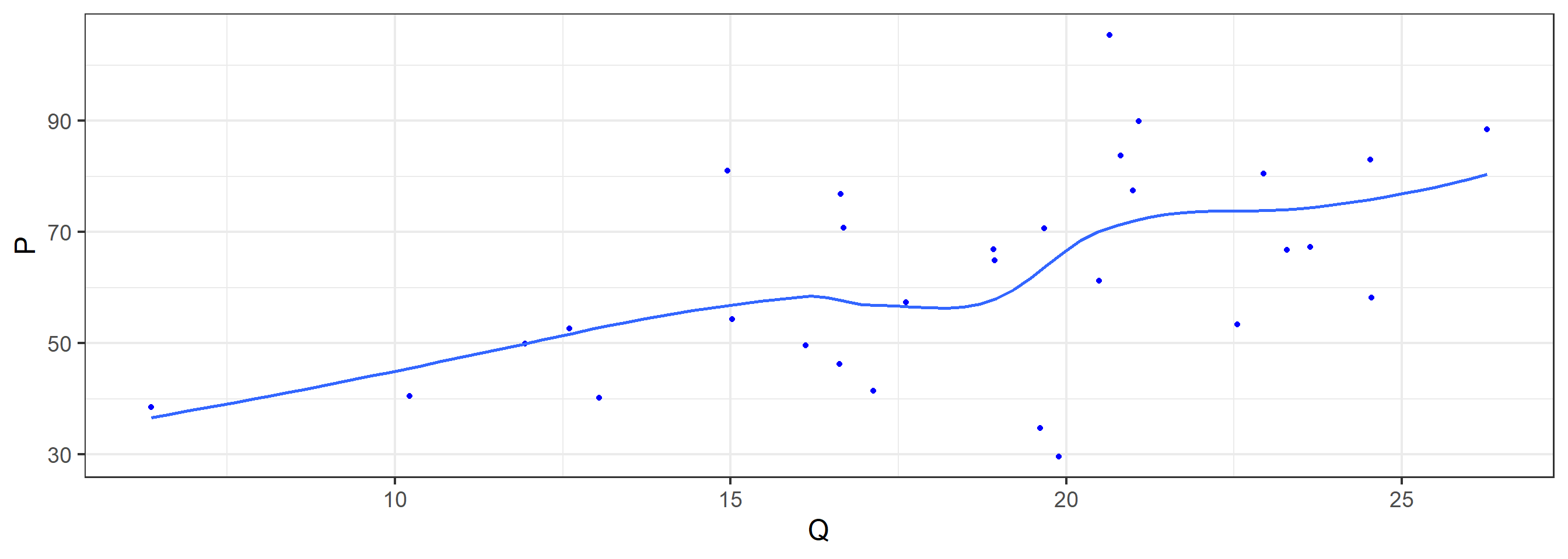
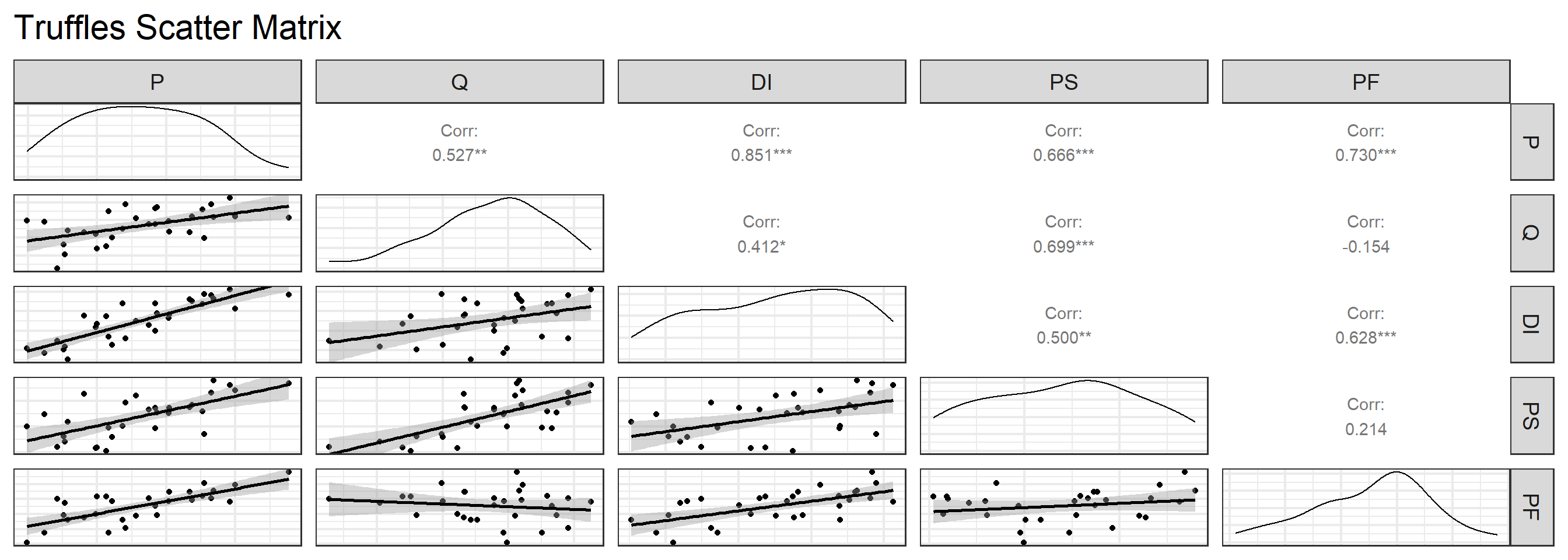
Truffles are delicious food materials. They are edible fungi that grow below the ground. Consider a supply and demand model for truffles:

\[ \begin{cases} \begin{align} \text { Demand: } & Q_{di}=\alpha_{1}+\alpha_{2} P_{i}+\alpha_{3} P S_{i}+\alpha_{4} D I_{i}+e_{d i} \\ \text { Supply: } & Q_{si}=\beta_{1}+\beta_{2} P_{i}+\beta_{3} P F_{i}+e_{s i}\\ \text { Equity: } & Q_{di}= Q_{si} \end{align} \end{cases} \]

where: - \(Q_i=\) the quantity of truffles traded in a particular marketplace; - \(P_i=\) the market price of truffles; - \(PS_i=\) the market price of a substitute for real truffles; - \(DI_i=\) per capita monthly disposable income of local residents; - \(PF_i=\) the price of a factor of production, which in this case is the hourly rental price of truffle-pigs used in the search process.

So, let us sum up this section with the truffles example.We will just walk through the sigle equation thought with the data set.And you should think about the difference between sigle equation model and SEM.

Model variables

松露案例：变量说明案例来源：Hill, R. C., W. E. Griffiths and G. C. Lim. Principles of Econometrics 4th Edition [M], Wiley, 2011. chpt 11。实例参考：PoE with R

The data set

The Scatter plot (P VS Q)

Figure 1

The Scatter matrix

Figure 2

The simple linear regression

Let’s start with the simplest linear regression model.

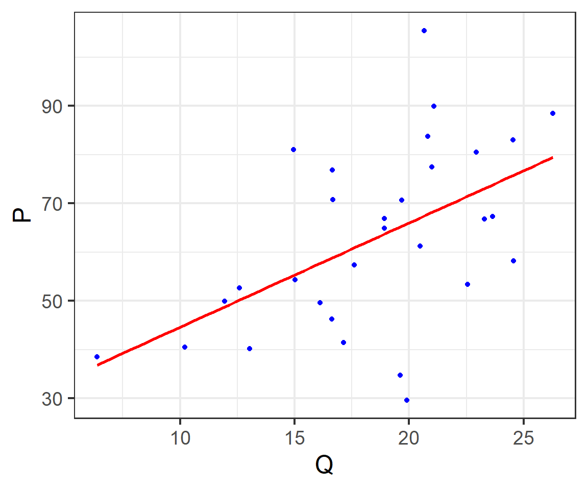
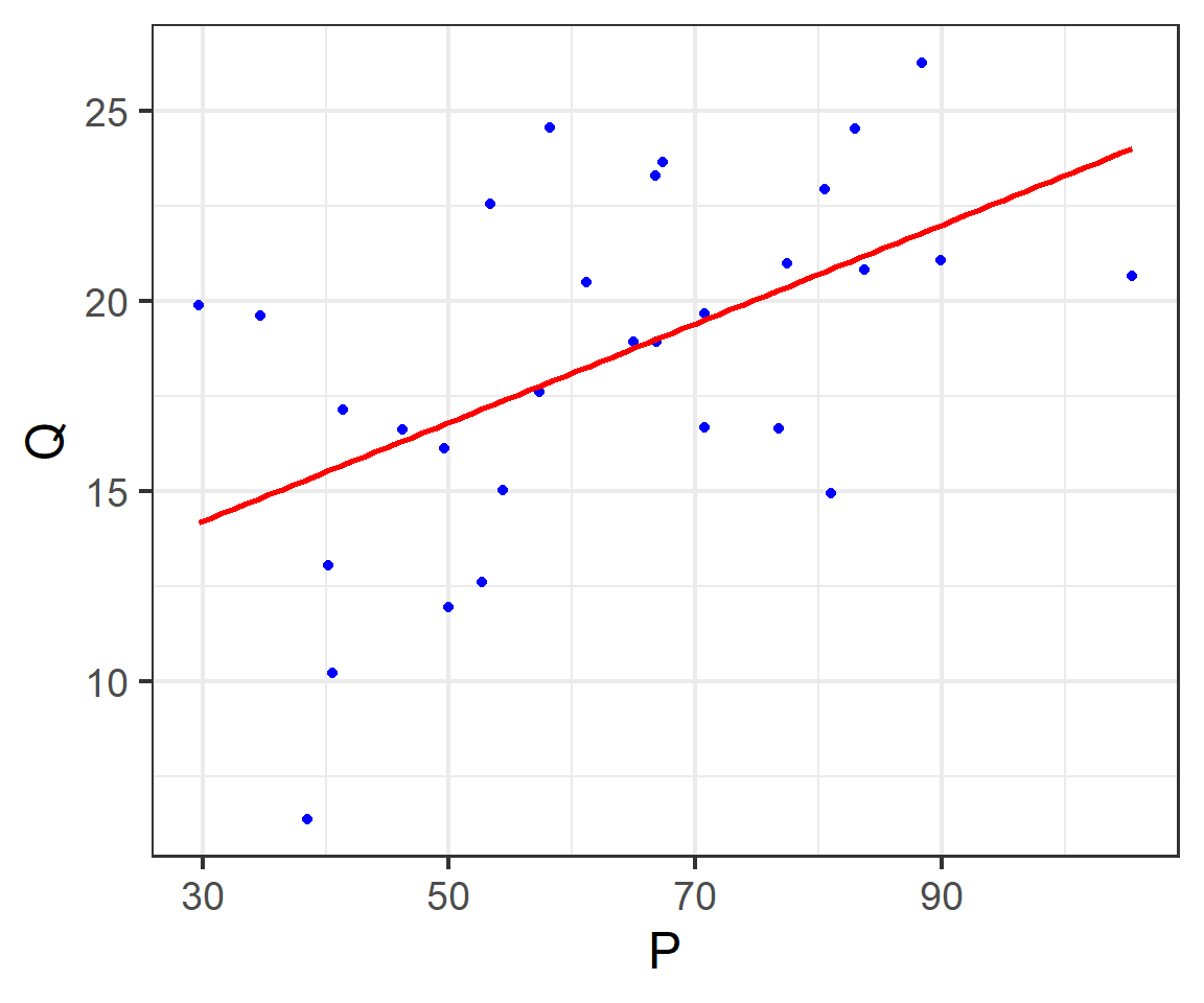
Generally, we use price (P) and output (Q) data to directly conduct simple linear regression modeling:

\[ \begin{cases} \begin{align} P & = \hat{\beta}_1+\hat{\beta}_2Q +e_1 && \text{(simple P model)}\\ Q & = \hat{\beta}_1+\hat{\beta}_2P +e_2 && \text{(simple Q model)} \end{align} \end{cases} \]

从最简单线性回归模型开始。通常我们会使用价格(P)和产量(Q)数据直接做简单线性回归建模：

The simple linear regression

As we all know, the linear regression of two variables is asymmetrical, so there is:

• the simple Price regression is:

\[ \begin{alignedat}{999} \begin{split} &\widehat{P}=&&+23.23&&+2.14Q_i\\ &(s)&&(12.3885)&&(0.6518)\\ &(t)&&(+1.87)&&(+3.28)\\ &(fit)&&R^2=0.2780&&\bar{R}^2=0.2522\\ &(Ftest)&&F^*=10.78&&p=0.0028 \end{split} \end{alignedat} \]

• the simple Quantity regression is:

\[ \begin{alignedat}{999} \begin{split} &\widehat{Q}=&&+10.31&&+0.13P_i\\ &(s)&&(2.5863)&&(0.0396)\\ &(t)&&(+3.99)&&(+3.28)\\ &(fit)&&R^2=0.2780&&\bar{R}^2=0.2522\\ &(Ftest)&&F^*=10.78&&p=0.0028 \end{split} \end{alignedat} \]

我们都知道，两个变量的线性回归是不对称的，因此有：

The sample regression line (SRL)

Figure 3: SRL of the Price model

Figure 4: SRL of the Quantity model

So, we can not distinguish the supply curve or the demand curve here.

The multi-variables regression model (1/2)

Of course, we can also use more independent variables X to build the regression models:

\[ \begin{cases} \begin{align} P & = \hat{\beta}_1+\hat{\beta}_2Q +\hat{\beta}_3DI+\hat{\beta}_2PS +e_1 && \text{(added P model)}\\ Q & = \hat{\beta}_1+\hat{\beta}_2P +\hat{\beta}_2PF+e_2 && \text{(added Q model)} \end{align} \end{cases} \]

Of course, we can also use more independent variables X to build the regression models.We tried hard to make these supply or demand equations more “reasonable” and “believable”.

The multi-variables regression model (2/2)

• Result of multi-vars Price regression model is:

\[ \begin{alignedat}{999} \begin{split} &\widehat{P}=&&-48.68&&+2.05Q_i&&+3.16DI_i\\ &(s)&&(5.0047)&&(0.2731)&&(1.1409)\\ &(t)&&(-9.73)&&(+7.50)&&(+2.77)\\ &(cont.)&&+0.36PS_i&&+2.39PF_i &&\\ &(s)&&(0.2674)&&(0.2184) &&\\ &(t)&&(+1.36)&&(+10.96) &&\\ &(fit)&&R^2=0.9658&&\bar{R}^2=0.9603 &&\\ &(Ftest)&&F^*=176.23&&p=0.0000 && \end{split} \end{alignedat} \]

• Result of multi-vars Quantity regression model:

\[ \begin{alignedat}{999} \begin{split} &\widehat{Q}=&&+18.88&&+0.34P_i&&-0.40DI_i\\ &(s)&&(2.3480)&&(0.0451)&&(0.5238)\\ &(t)&&(+8.04)&&(+7.50)&&(-0.77)\\ &(cont.)&&+0.08PS_i&&-0.96PF_i &&\\ &(s)&&(0.1115)&&(0.0918) &&\\ &(t)&&(+0.71)&&(-10.51) &&\\ &(fit)&&R^2=0.9069&&\bar{R}^2=0.8920 &&\\ &(Ftest)&&F^*=60.88&&p=0.0000 && \end{split} \end{alignedat} \]

However, we know that in the demand-supply SEM, reverse causility effect will existbetween the price and quantity variables.So, these simple OLS estimates are unreliable with our intuition.

18.2 Notations and Definitions

In this section, I will give you some important definition and notations about SEM.

Structural SEM

Algebraic expression (A)

Structural equations: System of equations that directly characterize economic structure or behavior.

The algebraic expression of structural SEM is：

\[ \begin{cases} \begin{alignat}{5} Y_{t1}&= & &+\gamma_{21}Y_{t2}+&\cdots &+\gamma_{m1}Y_{tm} & +\beta_{11}X_{1t}+\beta_{21}X_{t2} &+\cdots+\beta_{k1}X_{tk} &+\varepsilon_{t1} \\ Y_{t2}&=&\gamma_{12}Y_{t1} &+ & \cdots &+\gamma_{m2}Y_{tm}&+\beta_{12}X_{t1}+\beta_{22}X_{t2} &+\cdots+\beta_{k2}X_{tk} &+\varepsilon_{t2}\\ & \vdots &\vdots &&\vdots &&\vdots \\ Y_{tm}&=&\gamma_{1m}Y_{t1}&+\gamma_{2m}Y_{t2}+& \cdots & &+\beta_{1m}X_{t1} +\beta_{2m}X_{t2} &+\cdots+\beta_{km}X_{tk} &+\varepsilon_{tm} \end{alignat} \end{cases} \]

algebraic /ˌældʒɪˈbreɪɪk/In fact, all examples we have seen in the former section are structural SEM.___So we donote the generalized algebraic expression of structural SEM as follows.

Structural coefficients

Structural coefficients: Parameters in structural equation that represents an economic outcome or behavioral relationship, including:

\[ \begin{cases} \begin{alignat}{5} Y_{t1}&= & &+\gamma_{21}Y_{t2}+&\cdots &+\gamma_{m1}Y_{tm} & +\beta_{11}X_{1t}+\beta_{21}X_{t2} &+\cdots+\beta_{k1}X_{tk} &+\varepsilon_{t1} \\ Y_{t2}&=&\gamma_{12}Y_{t1} &+ & \cdots &+\gamma_{m2}Y_{tm}&+\beta_{12}X_{t1}+\beta_{22}X_{t2} &+\cdots+\beta_{k2}X_{tk} &+\varepsilon_{t2}\\ & \vdots &\vdots &&\vdots &&\vdots \\ Y_{tm}&=&\gamma_{1m}Y_{t1}&+\gamma_{2m}Y_{t2}+& \cdots & &+\beta_{1m}X_{t1} +\beta_{2m}X_{t2} &+\cdots+\beta_{km}X_{tk} &+\varepsilon_{tm} \end{alignat} \end{cases} \]

• Endogenous structural coefficients: \(\gamma_{11}, \gamma_{21},\cdots, \gamma_{m1}; \cdots; \gamma_{1m}, \gamma_{2m},\cdots, \gamma_{mm}\)

• Exogenous structural coefficients: \(\beta_{11}, \beta_{21},\cdots, \beta_{m1}; \cdots; \beta_{1m}, \beta_{2m},\cdots, \beta_{mm};\)

Firstly, let’s define the structural coefficients.Structural coefficients are Parameters in structural SEM that represents an economic outcome or behavioral relationship, including Endogenous structural coefficients (here denoted as …) and Exogenous structural coefficients (here denoted as …) .

Structural variables

• Endogenous variables: Variables determined by the model.

• Predetermined variables：Variables which values are not determined by the model in the current time period.

\[ \begin{cases} \begin{alignat}{5} Y_{t1}&= & &+\gamma_{21}Y_{t2}+&\cdots &+\gamma_{m1}Y_{tm} & +\beta_{11}X_{1t}+\beta_{21}X_{t2} &+\cdots+\beta_{k1}X_{tk} &+\varepsilon_{t1} \\ Y_{t2}&=&\gamma_{12}Y_{t1} &+ & \cdots &+\gamma_{m2}Y_{tm}&+\beta_{12}X_{t1}+\beta_{22}X_{t2} &+\cdots+\beta_{k2}X_{tk} &+\varepsilon_{t2}\\ & \vdots &\vdots &&\vdots &&\vdots \\ Y_{tm}&=&\gamma_{1m}Y_{t1}&+\gamma_{2m}Y_{t2}+& \cdots & &+\beta_{1m}X_{t1} +\beta_{2m}X_{t2} &+\cdots+\beta_{km}X_{tk} &+\varepsilon_{tm} \end{alignat} \end{cases} \]

Endogenous variables:

• Such as: \(Y_{t1};Y_{t2}; \cdots; Y_{tm}\)

Predetermined variables:

• Such as: \(X_{..}\)

Another important concept is the structural variable, which includes endogenouse variable and predeterminded variable.Endogenous variables are Variables determined by the model.Predetermined variables are Variables which values are not determined by the model in the current time period.We assumed the endogenous variables in this SEM includes all Y_ts, and the predeterminded vairiables include all X_ts.

Predetermined variables

Predetermined variables: Variables which values are not determined by the model in the current time period, including:

• the exogenous variables

• the lagged endogenous variables.

\[ \begin{cases} \begin{alignat}{5} Y_{t1}&= & &+\gamma_{21}Y_{t2}+&\cdots &+\gamma_{m1}Y_{tm} & +\beta_{11}X_{1t}+\beta_{21}X_{t2} &+\cdots+\beta_{k1}X_{tk} &+\varepsilon_{t1} \\ Y_{t2}&=&\gamma_{12}Y_{t1} &+ & \cdots &+\gamma_{m2}Y_{tm}&+\beta_{12}X_{t1}+\beta_{22}X_{t2} &+\cdots+\beta_{k2}X_{tk} &+\varepsilon_{t2}\\ & \vdots &\vdots &&\vdots &&\vdots \\ Y_{tm}&=&\gamma_{1m}Y_{t1}&+\gamma_{2m}Y_{t2}+& \cdots & &+\beta_{1m}X_{t1} +\beta_{2m}X_{t2} &+\cdots+\beta_{km}X_{tk} &+\varepsilon_{tm} \end{alignat} \end{cases} \]

You should remind that the predetermined variables consist of both the exogenous variables and thelagged endogenous variables.

Predetermined variables

• Exogenous variables: The variables not determined by the model, neither in the current period nor in the lagged period.

• Lagged endogenous variables: The lag variable of the endogenous variable in the current period。

current period exogenous: - \(X_{t1}, X_{t2},\cdots, X_{tk}\) .

lagged period exdogenous: - lagged from \(X_{t1}\) : \(X_{t-1,1}; X_{t-2,1};\cdots; X_{t-(T-1),1}\) - and lagged from \(X_{tk}\) : \(X_{t-1,k}; X_{t-2,k};\cdots; X_{t-(T-1),k}\) - \(\cdots\)

lagged endogenous: - lagged from \(Y_{t1}\) : \(Y_{t-1,1}; Y_{t-2,1}; \cdots, Y_{t-(T-1),1}\) - and lagged from \(Y_{tm}\) ： \(Y_{t-1,m}; Y_{t-2,m}; \cdots;Y_{t-(T-1),m}\) - \(\cdots\)

So, you may get two types Exogenous variables, which are current period exogenous, such as all X_ts, and Lagged endogenous variables, such as all X_t-s.

Predetermined coefficients

Predetermined coefficients: coefficients before predetermined variables.

\[ \begin{cases} \begin{alignat}{5} Y_{t1}&= & &+\gamma_{21}Y_{t2}+&\cdots &+\gamma_{m1}Y_{tm} & +\beta_{11}X_{1t}+\beta_{21}X_{t2} &+\cdots+\beta_{k1}X_{tk} &+\varepsilon_{t1} \\ Y_{t2}&=&\gamma_{12}Y_{t1} &+ & \cdots &+\gamma_{m2}Y_{tm}&+\beta_{12}X_{t1}+\beta_{22}X_{t2} &+\cdots+\beta_{k2}X_{tk} &+\varepsilon_{t2}\\ & \vdots &\vdots &&\vdots &&\vdots \\ Y_{tm}&=&\gamma_{1m}Y_{t1}&+\gamma_{2m}Y_{t2}+& \cdots & &+\beta_{1m}X_{t1} +\beta_{2m}X_{t2} &+\cdots+\beta_{km}X_{tk} &+\varepsilon_{tm} \end{alignat} \end{cases} \]

Such as: \(\beta_{11}, \beta_{21},\cdots, \beta_{12}; \cdots; \beta_{k2}, \beta_{1m},\cdots, \beta_{km}\)

Of course, we may denote coefficients before predetermined variables as Predetermined coefficients.

Algebraic expression (B)

By simple transformation, the algebraic expression of SEM can also show as:

\[ A: \begin{cases} \begin{alignat}{5} Y_{t1}&= & &+\gamma_{21}Y_{t2}+&\cdots &+\gamma_{m1}Y_{tm} & +\beta_{11}X_{1t}+\beta_{21}X_{t2} &+\cdots+\beta_{k1}X_{tk} &+\varepsilon_{t1} \\ Y_{t2}&=&\gamma_{12}Y_{t1} &+ & \cdots &+\gamma_{m2}Y_{tm}&+\beta_{12}X_{t1}+\beta_{22}X_{t2} &+\cdots+\beta_{k2}X_{tk} &+\varepsilon_{t2}\\ & \vdots &\vdots &&\vdots &&\vdots \\ Y_{tm}&=&\gamma_{1m}Y_{t1}&+\gamma_{2m}Y_{t2}+& \cdots & &+\beta_{1m}X_{t1} +\beta_{2m}X_{t2} &+\cdots+\beta_{km}X_{tk} &+\varepsilon_{tm} \end{alignat} \end{cases} \]

\[ B: \begin{cases} \begin{alignat}{5} \gamma_{11}Y_{t1} &+ \gamma_{21}Y_{t2}&+\cdots &+\gamma_{m-1,1}Y_{t,m-1} &+\gamma_{m1}Y_{tm} & +\beta_{11}X_{t1}+\beta_{21}X_{t2} &+\cdots+\beta_{k1}X_{tk} &=\varepsilon_{t1} \\ \gamma_{12}Y_{t1} &+\gamma_{22}Y_{t2} &+ \cdots&+\gamma_{m-1,2}Y_{t,m-1} &+\gamma_{m2}Y_{tm}&+\beta_{12}X_{t1}+\beta_{22}X_{t2} &+\cdots+\beta_{k2}X_{tk} &= \varepsilon_{t2}\\ & \vdots &\vdots &&\vdots &&\vdots \\ \gamma_{1m}Y_{t1}&+\gamma_{2m}Y_{t2}&+ \cdots &+\gamma_{m-1,m}Y_{t,m-1} & +\gamma_{mm}Y_{tm} &+\beta_{1m}X_{t1} +\beta_{2m}X_{t2} &+\cdots+\beta_{km}X_{tk} &=\varepsilon_{tm} \end{alignat} \end{cases} \]

By simple transformation, we can also obtain another algebraic expression (B) of SEM as show in this slide.

Matrix expression (1/2)

With the Matrix language, the matrix expression of SEM was noted as:

\[ \begin{equation} \begin{bmatrix} Y_1 & Y_2 & \cdots & Y_m \\ \end{bmatrix} _t \begin{bmatrix} \gamma_{11} & \gamma_{12} & \cdots & \gamma_{1m} \\ \gamma_{21} & \gamma_{22} & \cdots & \gamma_{2m} \\ \cdots & \cdots & \cdots & \cdots \\ \gamma_{m1} & \gamma_{m2} & \cdots & \gamma_{mm} \\ \end{bmatrix} + \\ \begin{bmatrix} X_1 & X_2 & \cdots & X_m \\ \end{bmatrix} _t \begin{bmatrix} \beta_{11} & \beta_{12} & \cdots & \beta_{1m} \\ \beta_{21} & \beta_{22} & \cdots & \beta_{2m} \\ \cdots & \cdots & \cdots & \cdots\\ \beta_{k1} & \beta_{k2} & \cdots & \beta_{km} \\ \end{bmatrix} \\ = \begin{bmatrix} \varepsilon_1 & \varepsilon_2 & \cdots & \varepsilon_m \\ \end{bmatrix} _t \end{equation} \]

Here, we arranged the matrix expression of SEM based on former algebraic expression B.

Matrix expression (2/2)

For Simplicity, we can generized the matrix expression of SEM :

\[ \begin{aligned} & \boldsymbol{y^{\prime}_t} \boldsymbol{\Gamma} &+ & \boldsymbol{x^{\prime}_t} \boldsymbol{B} &= & \boldsymbol{{\varepsilon^{\prime}_t}} \\ &(1 \ast m)(m \ast m) & & (1 \ast k)(k \ast m) & & (1 \ast m) \end{aligned} \]

where：

• Bold upper letter and greek means a matrix

• Bold lower letter and greek means a column vector

For Simplicity, we can generized the matrix expression of SEM as follow.> we should remind that：- the dimension of the vector and matrix is important;- and matrix compatibility /kəmˌpætəˈbɪləti/ is needed in matrix calculation.

Endogenous coefficients matrix

For the Endogenous parameter matrix \(\boldsymbol{\Gamma}\) , To ensure that each equation has a dependent variable, then the matrix \(\boldsymbol{\Gamma}\) each column has at least one element of 1

\[ \begin{equation} \boldsymbol{\Gamma} = \begin{bmatrix} \gamma_{11} & \gamma_{12} & \cdots & \gamma_{1m} \\ \gamma_{21} & \gamma_{22} & \cdots & \gamma_{2m} \\ \cdots & \cdots & \cdots & \cdots \\ \gamma_{m1} & \gamma_{m2} & \cdots & \gamma_{mm} \\ \end{bmatrix} \\ \text{if }\Rightarrow \begin{bmatrix} \gamma_{11} & \gamma_{12} & \cdots & \gamma_{1m} \\ 0 & \gamma_{22} & \cdots & \gamma_{2m} \\ \cdots & \cdots & \cdots & \cdots \\ 0 & 0 & \cdots & \gamma_{mm} \\ \end{bmatrix} \end{equation} \]

\[ \begin{cases} \begin{aligned} y_{1t} &=& f_{1}\left(\mathbf{x}_{t}\right)+\varepsilon_{t1} \\ y_{2t} &=& f_{2}\left(y_{t1}, \mathbf{x}_{t}\right)+\varepsilon_{t2} \\ & \vdots & \vdots \\ y_{mt} &=& f_{m}\left(y_{t1}, y_{t2}, \ldots, \mathbf{x}_{t}\right)+\varepsilon_{mt} \end{aligned} \end{cases} \]

• If matrix \(\boldsymbol{\Gamma}\) is upper triangular matrix, then the SEM is a recursive model system.

• For the SEM solution to exist, \(\boldsymbol{\Gamma}\) must be nonsingular.

Now, let’s focus the Endogenous parameter matrix firstly.

Exdogenous coefficients matrix

The Exogenous coefficients matrix \(\boldsymbol{B}\) ：

\[ \begin{equation} \boldsymbol{B} = \begin{bmatrix} \beta_{11} & \beta_{12} & \cdots & \beta_{1m} \\ \beta_{21} & \beta_{22} & \cdots & \beta_{2m} \\ \cdots & \cdots & \cdots & \cdots\\ \beta_{k1} & \beta_{k2} & \cdots & \beta_{km} \\ \end{bmatrix} \end{equation} \]

Here is the The Exogenous coefficients matrix.You should pay attention that the first column if SEM contains intercepts.

Reduced SEM

Algebraic expression

Reduced equations: The equation expresses an endogenous variable with all the predetermined variables and the stochastic disturbances.

\[ \begin{cases} \begin{alignat}{5} Y_{t1}&= & +\pi_{11}X_{t1}+\pi_{21}X_{t2} &+\cdots+\pi_{k1}X_{tk} & + v_{t1} \\ Y_{t2}&=&+\pi_{12}X_{t1}+\pi_{22}X_{t2} &+\cdots+\pi_{k2}X_{tk} & + v_{t2}\\ & \vdots &\vdots &&\vdots & \\ Y_{tm}&=&+\pi_{1m}X_{t1} +\pi_{2m}X_{t2} &+\cdots+\pi_{km}X_{tk} & + v_{tm} \end{alignat} \end{cases} \]

As you see, we know well with the structural SEMs because we have learned thess models in the economic textbooks.Now, we will go ahead to the important concept of reduced SEM.___So, a reduced equation is one that expresses an endogenous variable solely in terms of the predetermined variables and the stochastic disturbances.We denoted the reduced SEM as follows.

Reduced coefficients and disturbance

• Reduced coefficients: parameters in the reduced SEM.

• Reduced disturbance: stochastic disturbance terms in the reduced SEM.

\[ \begin{cases} \begin{alignat}{5} Y_{t1}&= & +\pi_{11}X_{t1}+\pi_{21}X_{t2} &+\cdots+\pi_{k1}X_{tk} & + v_{t1} \\ Y_{t2}&=&+\pi_{12}X_{t1}+\pi_{22}X_{t2} &+\cdots+\pi_{k2}X_{tk} & + v_{t2}\\ & \vdots &\vdots &&\vdots & \\ Y_{tm}&=&+\pi_{1m}X_{t1} +\pi_{2m}X_{t2} &+\cdots+\pi_{km}X_{tk} & + v_{tm} \end{alignat} \end{cases} \]

Reduced coefficients: - \(\pi_{11},\pi_{21},\cdots, \pi_{k1}\) - \(\pi_{1m},\pi_{2m},\cdots, \pi_{km}\) .

Reduced disturbance: - \(v_{1},v_2,\cdots, v_m\) 。

Hence, we induce the concepts of Reduced coefficients and Reduced disturbance.- Reduced coefficients are parameters in the reduced SEM, such as all \(\pi_{km}\)s.- Reduced disturbance: stochastic disturbance terms in the reduced SEM, such as all \(v_{m}\)s.

Matrix expression (1/2)

\[ \begin{cases} \begin{alignat}{5} Y_{t1}&= & +\pi_{11}X_{t1}+\pi_{21}X_{t2} &+\cdots+\pi_{k1}X_{tk} & + v_{t1} \\ Y_{t2}&=&+\pi_{12}X_{t1}+\pi_{22}X_{t2} &+\cdots+\pi_{k2}X_{tk} & + v_{t2}\\ & \vdots &\vdots &&\vdots & \\ Y_{tm}&=&+\pi_{1m}X_{t1} +\pi_{2m}X_{t2} &+\cdots+\pi_{km}X_{tk} & + v_{tm} \end{alignat} \end{cases} \]

For this algebraic reduced SEM, we can note its matrix form as:

\[ \begin{equation} \begin{bmatrix} Y_1 & Y_2 & \cdots & Y_m \\ \end{bmatrix} _t = \\ \begin{bmatrix} X_1 & X_2 & \cdots & X_m \\ \end{bmatrix} _t \begin{bmatrix} \pi_{11} & \pi_{12} & \cdots & \pi_{1m} \\ \pi_{21} & \pi_{22} & \cdots & \pi_{2m} \\ \cdots & \cdots & \cdots & \cdots \\ \pi_{m1} & \pi_{m2} & \cdots & \pi_{mm} \\ \end{bmatrix} + \begin{bmatrix} v_1 & v_2 & \cdots & v_m \\ \end{bmatrix} _t \end{equation} \]

Also, we can denote the matrix form of the reduced SEM as below.

Matrix expression (2/2)

For simplicity, the matrix expression of reduced SEM can be noted further.

\[ \begin{aligned} & \boldsymbol{y^{\prime}_t} & = &\boldsymbol{x^{\prime}_t} \boldsymbol{\Pi} & + & \boldsymbol{{v^{\prime}_t}} \\ &(1 \ast m) & & (1 \ast k)(k \ast m) & & (1 \ast m) \end{aligned} \]

• the reduced coefficients matrix is :

\[ \begin{equation} \boldsymbol{\Pi} = \begin{bmatrix} \pi_{11} & \pi_{12} & \cdots & \pi_{1m} \\ \pi_{21} & \pi_{22} & \cdots & \pi_{2m} \\ \cdots & \cdots & \cdots & \cdots \\ \pi_{m1} & \pi_{m2} & \cdots & \pi_{mm} \\ \end{bmatrix} \end{equation} \]

• the reduced disturbances vector is:

\[ \begin{equation} \boldsymbol{{v^{\prime}_t}}= \begin{bmatrix} v_1 & v_2 & \cdots & v_m \\ \end{bmatrix}_t \end{equation} \]

Structural VS Reduced SEM

The two systems

We can induce Reduced Equations from Structural Equations:

\[ \begin{cases} \begin{alignat}{5} Y_{t1}&= & &+\gamma_{21}Y_{t2}+&\cdots &+\gamma_{m1}Y_{tm} & +\beta_{11}X_{1t}+\beta_{21}X_{t2} &+\cdots+\beta_{k1}X_{tk} &+\varepsilon_{t1} \\ Y_{t2}&=&\gamma_{12}Y_{t1} &+ & \cdots &+\gamma_{m2}Y_{tm}&+\beta_{12}X_{t1}+\beta_{22}X_{t2} &+\cdots+\beta_{k2}X_{tk} &+\varepsilon_{t2}\\ & \vdots &\vdots &&\vdots &&\vdots \\ Y_{tm}&=&\gamma_{1m}Y_{t1}&+\gamma_{2m}Y_{t2}+& \cdots & &+\beta_{1m}X_{t1} +\beta_{2m}X_{t2} &+\cdots+\beta_{km}X_{tk} &+\varepsilon_{tm} \end{alignat} \end{cases} \]

\[ \Rightarrow\begin{cases} \begin{alignat}{5} Y_{t1}&= & +\pi_{11}X_{t1}+\pi_{21}X_{t2} &+\cdots+\pi_{k1}X_{tk} & + v_{t1} \\ Y_{t2}&=&+\pi_{12}X_{t1}+\pi_{22}X_{t2} &+\cdots+\pi_{k2}X_{tk} & + v_{t2}\\ & \vdots &\vdots &&\vdots & \\ Y_{tm}&=&+\pi_{1m}X_{t1} +\pi_{2m}X_{t2} &+\cdots+\pi_{km}X_{tk} & + v_{tm} \end{alignat} \end{cases} \]

Untill now, we have two notation systems. one is the structural SEM, and the other is the reduced SEM.So, Why we need these two notation systems ?And what is the relationship between these two notation systems ?A short answer is that we can deduce the structural parameters with the reduced coefficients.

Coefficients

The Structural SEM :

\[ \begin{aligned} \boldsymbol{y^{\prime}_t} \boldsymbol{\Gamma} + \boldsymbol{x^{\prime}_t} \boldsymbol{B} = \boldsymbol{{\varepsilon^{\prime}_t}} \end{aligned} \]

The Reduced SEM:

\[ \begin{aligned} \boldsymbol{y^{\prime}_t} = \boldsymbol{x^{\prime}_t} \boldsymbol{\Pi} + \boldsymbol{{v^{\prime}_t}} \end{aligned} \]

• where:

\[ \begin{align} \boldsymbol{\Pi} &= - \boldsymbol{B} \boldsymbol{\Gamma^{-1}}\\ \boldsymbol{{v^{\prime}_t}} &= \boldsymbol{{\varepsilon^{\prime}_t}} \boldsymbol{\Gamma}^{-1} \end{align} \]

• and:

\[ \begin{equation} \boldsymbol{\Gamma} = \begin{bmatrix} \gamma_{11} & \gamma_{12} & \cdots & \gamma_{1m} \\ \gamma_{21} & \gamma_{22} & \cdots & \gamma_{2m} \\ \cdots & \cdots & \cdots & \cdots \\ \gamma_{m1} & \gamma_{m2} & \cdots & \gamma_{mm} \\ \end{bmatrix} \end{equation} \]

This slide shows the relationship between the structural SEM and the reduced SEM.And the reduced coefficients equals negetive B times the inverse matrix of structural pars.

\[ \begin{aligned}& \boldsymbol{y^{\prime}_t} & = &-\boldsymbol{x^{\prime}_t} \boldsymbol{B} \boldsymbol{\Gamma^{-1}} & + & \boldsymbol{{\varepsilon^{\prime}_t}} \boldsymbol{\Gamma}^{-1} \\&(1 \ast m) & & (1 \ast k)(k \ast m)(m \ast m) & & (1 \ast m)(m \ast m)\end{aligned} \]

Moments

Now we concern the first and second moments of the disturbance:

• first , let us assumed the moments of structural disturbances satisfy:

\[ \begin{align} \mathbf{E[\varepsilon_t | x_t]} &= \mathbf{0} \\ \mathbf{E[\varepsilon_t \varepsilon^{\prime}_t |x_t]} &= \mathbf{\Sigma} \\ E\left[\boldsymbol{\varepsilon}_{t} \boldsymbol{\varepsilon}_{s}^{\prime} | \mathbf{x}_{t}, \mathbf{x}_{s}\right] &=\mathbf{0}, \quad \forall t, s \end{align} \]

• then, we can prove that the reduced disturbances satify:

\[ \begin{align} E\left[\mathbf{v}_{t} | \mathbf{x}_{t}\right] &=\left(\mathbf{\Gamma}^{-1}\right)^{\prime} \mathbf{0}=\mathbf{0} \\ E\left[\mathbf{v}_{t} \mathbf{v}_{t}^{\prime} | \mathbf{x}_{t}\right] &=\left(\mathbf{\Gamma}^{-1}\right)^{\prime} \mathbf{\Sigma} \mathbf{\Gamma}^{-1}=\mathbf{\Omega} \\ \text{where: }\mathbf{\Sigma} &=\mathbf{\Gamma}^{\prime} \mathbf{\Omega} \mathbf{\Gamma} \end{align} \]

This slide shows the first and second moments of the disturbance on both structural and reduced SEM.First , let us assumed the moments of structural disturbances satisfy following moment conditions. which means that the structural disturbances are drawn from an M-variate distribution with zero conditional expectation and zero covariance.Then, we can prove that the reduced disturbances will also be zero conditional expectation and its variance-covariance matrix equals omega.Finaly, we know the relationship between these two variance-covariance matrix.We denote the relationship as Sigma equals transpose Gamma times Omega times Gamma.

Useful expression* (1/2)

In a sample of data, each joint observation will be one row in a data matrix ( with \(T\) observations):

\[ \begin{align} \left[\begin{array}{lll}{\mathbf{Y}} & {\mathbf{X}} & {\mathbf{E}}\end{array}\right]=\left[\begin{array}{ccc}{\mathbf{y}_{1}^{\prime}} & {\mathbf{x}_{1}^{\prime}} & {\boldsymbol{\varepsilon}_{1}^{\prime}} \\ {\mathbf{y}_{2}^{\prime}} & {\mathbf{x}_{2}^{\prime}} & {\boldsymbol{\varepsilon}_{2}^{\prime}} \\ {\vdots} & {} \\ {\mathbf{y}_{T}^{\prime}} & {\mathbf{x}_{T}^{\prime}} & {\boldsymbol{\varepsilon}_{T}^{\prime}}\end{array}\right] \end{align} \]

then the structural SEM is:

\[ \begin{align} \mathbf{Y} \mathbf{\Gamma}+\mathbf{X} \mathbf{B}=\mathbf{E} \end{align} \]

the first and second moment of structural disturbances is:

\[ \begin{align} E[\mathbf{E} | \mathbf{X}] &=\mathbf{0} \\ E\left[(1 / T) \mathbf{E}^{\prime} \mathbf{E} | \mathbf{X}\right] &=\mathbf{\Sigma} \end{align} \]

The next two slides will show us some useful relationships under sample data set.I will not discuss them here, and you should try to learn this content by yourself.

Useful expression*

Assume that:

\[ \begin{align} (1 / T) \mathbf{X}^{\prime} \mathbf{X} & \rightarrow \mathbf{Q} \text{ ( a finite positive definite matrix)} \\ (1 / T) \mathbf{X}^{\prime} \mathbf{E} & \rightarrow \mathbf{0} \end{align} \]

then the reduced SEM can be noted as:

\[ \begin{align} \mathbf{Y} & =\mathbf{X} \boldsymbol{\Pi}+\mathbf{V} && \leftarrow \mathbf{V}=\mathbf{E} \mathbf{\Gamma}^{-1} \end{align} \]

And we may have following useful results：

\[ \begin{align} \frac{1}{T} \begin{bmatrix} {\mathbf{Y}^{\prime}} \\ {\mathbf{X}^{\prime}} \\ {\mathbf{V}^{\prime}} \end{bmatrix} \begin{bmatrix} {\mathbf{Y}} & {\mathbf{X}} & {\mathbf{V}} \end{bmatrix} \quad \rightarrow \quad \begin{bmatrix} {\mathbf{I}^{\prime} \mathbf{Q} \mathbf{I}+\mathbf{\Omega}} & {\mathbf{I} \mathbf{I}^{\prime} \mathbf{Q}} & {\mathbf{\Omega}} \\ {\mathbf{Q} \mathbf{I}} & {\mathbf{Q}} & {\mathbf{0}^{\prime}} \\ {\mathbf{\Omega}} & {\mathbf{0}} & {\mathbf{\Omega}} \end{bmatrix} \end{align} \]

The next two slides will show us some useful relationships under sample data set.I will not discuss them here, and you should try to learn this content by yourself.

Case 1: Keynesian income model

Structural SEM

The Keynesian model of income determination (structural SEM):

\[ \begin{cases} \begin{align} C_t &= \beta_0+\beta_1Y_t+\varepsilon_t &&\text{(consumption function)}\\ Y_t &= C_t+I_t &&\text{(income equity)} \end{align} \end{cases} \]

So the structural SEM contains:

2 endogenous variables: - \(c_t;Y_t\)

1 predetermined variables:

• 1 exogenous variables: \(I_t\)

• 0 lagged endogenous variable.

Exercise: can you get the reduced SEM from this structural SEM ?

Now, I will show two cases to illustrate the relationship between the structural SEM and the reduced SEM. Here is the Keynesian model of income determination, and you know this is the structural SEM.So, can you deduce the reduced SEM from this structural SEM ?

Reduced SEM

We can get the reduced SEM from the former structural SEM and denoted (the right):

\[ \begin{cases} \begin{align} Y_t &=\frac{\beta_0}{1-\beta_1}+\frac{1}{1-\beta_1}I_t+\frac{\varepsilon_t}{1-\beta_1} \\ C_t &=\frac{\beta_0}{1-\beta_1}+\frac{\beta_1}{1-\beta_1}I_t+\frac{\varepsilon_t}{1-\beta_1} \end{align} \end{cases} \]

\[ \begin{cases} \begin{align} Y_t &= \pi_{11}+\pi_{21}I_t+v_{t1} \\ C_t &= \pi_{12}+\pi_{22}I_t+v_{t2} \end{align} \end{cases} \]

where:

\[ \begin{cases} \begin{alignat}{5} && \pi_{11} = \frac{\beta_0}{1-\beta_1}; \quad && \pi_{21} = \frac{\beta_0}{1-\beta_1}; \quad && v_{t1} = \frac{\varepsilon_t}{1-\beta_1};\\ && \pi_{12} = \frac{1}{1-\beta_1} ; \quad && \pi_{22} = \frac{\beta_1}{1-\beta_1} ; \quad && v_{t2} = \frac{\varepsilon_t}{1-\beta_1}; \end{alignat} \end{cases} \]

there are 2 structural coefficients \(\beta_0;\beta_1\) totally ； and 4 reduced coefficients \(\pi_{11},\pi_{21};\pi_{12},\pi_{22}\) (There are actually three only !)

Surely, We can get the reduced SEM from the former structural SEM with some simple algebraic calculation.Also, you can obtain the relationship between the structural parameters and the reduced coefficients.This is easy because the structural SEM contains only two equations and few structural parameters.

Case 2: Macroeconomic Model

Structural SEM

Consider the Small Macroeconomic Model (Structural SEM):

\[ \begin{cases} \begin{aligned} \text { consumption: } c_{t} &=\alpha_{0}+\alpha_{1} y_{t}+\alpha_{2} c_{t-1}+\varepsilon_{t, c} \\ \text { investment: } i_{t} &=\beta_{0}+\beta_{1} r_{t}+\beta_{2}\left(y_{t}-y_{t-1}\right)+\varepsilon_{t, j} \\ \text { demand: } y_{t} &=c_{t}+i_{t}+g_{t} \end{aligned} \end{cases} \]

where: \(c_t =\) consumption; \(y_t =\) output; \(i_t =\) investment; \(r_t =\) rate; \(g_t =\) government expenditure.

3 endogenous variables: \(c_t;i_t;Y_t\)

4 predetermined variables:

• 2 exogenous variables: \(r_t;g_t\) . - 2 lagged endogenous variables: \(y_{t-1};c_{t-1}\)

totally 6 strutural coefficients: \(\alpha_0,\alpha_1,\alpha_2;\beta_0,\beta_1,\beta_2;\)

So, let’s go ahead to more complex structural SEM with three equations.

Reduced SEM

We can get the reduced SEM from the former structural SEM: (HOW TO??)

\[ \begin{cases} \begin{align} c_{t} = & [{\alpha_{0}}{\left(1-\beta_{2}\right)}+\beta_{0} \alpha_{1}+\alpha_{1} \beta_{1} r_{t}+\alpha_{1} g_{t}+\alpha_{2}\left(1-\beta_{2}\right) c_{t-1}-\alpha_{1} \beta_{2} y_{t-1} \\ +&\left(1-\beta_{2}\right) \varepsilon_{t, c}+\alpha_{1} \varepsilon_{t, j}] /{\Lambda} \\ i_{t} = & [\alpha_{0} \beta_{2}+\beta_{0}\left(1-\alpha_{1}\right)+\beta_{1}\left(1-\alpha_{1}\right) r_{t}+\beta_{2} g_{t}+\alpha_{2} \beta_{2} c_{t-1}-\beta_{2}\left(1-\alpha_{1}\right) y_{t-1} \\ +&\beta_{2} \varepsilon_{t, c}+\left(1-\alpha_{1}\right) \varepsilon_{t, j}]/{\Lambda} \\ y_{t} = & [\alpha_{0}+\beta_{0}+\beta_{1} r_{t}+g_{t}+\alpha_{2} c_{t-1}-\beta_{2} y_{t-1} +\varepsilon_{t, c}+\varepsilon_{t, j}] /{\Lambda} \end{align} \end{cases} \]

where: \(\Lambda = 1- \alpha_1 -\beta_2\) 。For simplicity, denote the reduced SEM as:

\[ \begin{cases} \begin{aligned} c_{t} & = \pi_{11} +\pi_{21}r_t +\pi_{31}g_t +\pi_{41}c_{t-1} +\pi_{51}y_{t-1} +v_{t1} \\ i_{t} & = \pi_{12} +\pi_{22}r_t +\pi_{32}g_t +\pi_{42}c_{t-1} +\pi_{52}y_{t-1} +v_{t2} \\ i_{t} & = \pi_{13} +\pi_{23}r_t +\pi_{33}g_t +\pi_{43}c_{t-1} +\pi_{53}y_{t-1} +v_{t3} \end{aligned} \end{cases} \]

So we have 15 reduced coefficients totally!

With a little long time calculation, you can obtain the reduced SEM and also the relationship between the structural parameters and the reduced coefficients.Anyway, the calculation becomes complex and tedious for most of us.

Thinking

Thinking：

• What are the purposes of structural SEM and reduced SEM respectively?

• Note the consumption function (in structural SEM): the rate \(i_t\) does not impact the consumption \(c_t\) !

• It will be obvious from the reduced SEM that \(\frac{\Delta c_t}{\Delta r_t} = \frac{\alpha_1 \beta_1}{\Lambda}\)

• Note the consumption function (in structural SEM): What are the reasons for the impact of income \(y_t\) on consumption \(c_t\) ?

• It’s also easy to get the answer by transformation: \(\frac{\Delta c_t}{ \Delta y_t} = \frac{\Delta c_t / \Delta r_t}{\Delta y_t / \Delta r_t} = \frac{\alpha_1 \beta_1 / \Lambda}{ \beta_1 / \Lambda} = \alpha_1\)

So, we shoul rethink that What is the use of structural SEM and reduced SEM respectively?Can we relieve the works by using alternative approaches?

The relationship

According to the relationship between Structural SEM and Reduced SEM:

\[ \begin{aligned} \boldsymbol{y^{\prime}_t} = &-\boldsymbol{x^{\prime}_t} \boldsymbol{\Pi} + \boldsymbol{{v^{\prime}_t}} = -\boldsymbol{x^{\prime}_t} \boldsymbol{B} \boldsymbol{\Gamma^{-1}} + \boldsymbol{{\varepsilon^{\prime}_t}} \boldsymbol{\Gamma}^{-1} \end{aligned} \]

Then, the following matrixes can be easily obtained:

\[ \begin{align} \mathbf{y}^{\prime} & = \begin{bmatrix} c & i & y \end{bmatrix}\\ \boldsymbol{x}^{\prime} & = \begin{bmatrix} 1 & r & g & c_{-1} & y_{-1} \end{bmatrix} \end{align} \]

\[ \begin{align} \mathbf{B}= \begin{bmatrix} {-\alpha_{0}} & {-\beta_{0}} & {0} \\ {0} & {-\beta_{1}} & {0} \\ {0} & {0} & {-1} \\ {-\alpha_{2}} & {0} & {0} \\ {0} & {\beta_{2}} & {0} \end{bmatrix} \end{align} \]

\[ \begin{align} \Gamma &= \begin{bmatrix} {1} & {0} & {-1} \\ {0} & {1} & {-1} \\ {-\alpha_{1}} & {-\beta_{2}} & {1} \end{bmatrix} \\ \mathbf{\Gamma}^{-1} &=\frac{1}{\Lambda} \begin{bmatrix} {1-\beta_{2}} & {\beta_{2}} & {1} \\ {\alpha_{1}} & {1-\alpha_{1}} & {1} \\ {\alpha_{1}} & {\beta_{2}} & {1} \end{bmatrix} \end{align} \]

Here, we will obtain the reduced coefficients with matrix algebraic calculation.And you should first know the relationship between Structural SEM and Reduced SEM.Then, we write down the following vectors and matrixes. Y, X,Gamma, B, and inverse Gamma.Note that the first element of the vector X’ is constant one for the intercept in our equations.I think the difficulty in this calculation is the inverse of matrix Gamma.

Calculations

We can get the same answers: (It’s so easy!)

\[ \begin{align} \boldsymbol{\Pi=-B\Gamma^{-1}}=\frac{1}{\Lambda} \begin{bmatrix} {\alpha_{0}\left(1-\beta_{2}\right)+\beta_{0} \alpha_{1}} & {\alpha_{0} \beta_{2}+\beta_{0}\left(1-\alpha_{1}\right)} & {\alpha_{0}+\beta_{0}} \\ {\alpha_{1} \beta_{1}} & {\beta_{1}\left(1-\alpha_{1}\right)} & \beta_1 \\ {\alpha_{1}} & {\beta_{2}} & 1 \\ {\alpha_{2}\left(1-\beta_{2}\right)}& {\alpha_{2} \beta_{2}} & \alpha_2\\ {-\beta_{2} \alpha_{1}} & {-\beta_{2}\left(1-\alpha_{1}\right)} &-\beta_2 \end{bmatrix} \end{align} \]

\[ \begin{align} \mathbf{\Pi}^{\prime}=\frac{1}{\Lambda} \begin{bmatrix} \alpha_{0}\left(1-\beta_{2}\right)+\beta_{0} \alpha_{1} & \alpha_{1} \beta_{1} & \alpha_{1} & \alpha_{2}\left(1-\beta_{2}\right) & -\beta_{2} \alpha_{1} \\ \alpha_{0} \beta_{2}+\beta_{0}\left(1-\alpha_{1}\right) & \beta_{1}\left(1-\alpha_{1}\right) & \beta_{2} & \alpha_{2} \beta_{2} & -\beta_{2}\left(1-\alpha_{1}\right) \\ \alpha_{0}+\beta_{0} & \beta_{1} & 1 & \alpha_{2} & -\beta_{2} \end{bmatrix} \end{align} \]

• Where:

\[ \Lambda = 1- \alpha_1 -\beta_2 \]

• Remeber that:

\[ \begin{align} \mathbf{x}^{\prime} = \begin{bmatrix} 1 & r & g & c_{-1} & y_{-1} \end{bmatrix} \end{align} \]

Now, we know that the reduced coefficients matrix equal to negtive B times inverse Gamma.with the matrix agebraic caculation, we finally get the result here.And you can compare the transpose Pi with the former result.___So, Matrix calculation is a sharp knife, handy and sharp!You should practice by yourself at least once.

Supplement

Inverse matrix solution and procedure*

Use the elementary row operation (Gauss-Jordan) to find the inverse matrix:

1. Construct augmented matrix

2. Transform the augmented matrix for many times until the goal is achieved.

Use cofactor, algebraic cofactor and adjoint matrix to get the inverse matrix:

1. Calculate cofactor matrix and algebraic cofactor matrix;

2. Calculate adjoint matrix: it is the transpose of the cofactor matrix;

3. Calculate the determinant of original matrix : each element of top row in the original matrix is multiplied by its corresponding top row element in the “cofactor matrix”;

4. Calculated the inverse matrix: 1/ determinant \(\times\) adjoint matrix

This slide gives you the solution and procedure to obtain the inverse matrix.And please try to practice by yourself.A.用初等行运算（高斯－若尔当）来求逆矩阵：1. 构造增广矩阵2. 对增广矩阵进行多次变换，直至达到目标。
B.用余子式、代数余子式和伴随矩阵来求逆矩阵1. 计算余子式矩阵和代数余子式矩阵2. 计算伴随矩阵：就是代数余子式矩阵的转置3. 计算原矩阵行列式：原矩阵顶行的每个元素乘以其对应”代数余子式矩阵”顶行元素。4. 计算得出逆矩阵：1/行列式 X 伴随矩阵

18.3 Is the OLS Method Still applicable ?

In this section, we will discuss the problems with the SEM by using OLS method directly.

Endogenous variable problem (1/2)

Consider Keynes’s model of income determination, We will be able to show that \(Y_t\) and \(u_t\) will be correlated, thus violating the CLRM A2 assumption.

\[ \begin{cases} \begin{align} C_t &= \beta_0+\beta_1Y_t+u_t &(0<\beta_1<1) &&\text{( consumption function)}\\ Y_t &= C_t+I_t & &&\text{(Income Identity)} \end{align} \end{cases} \]

By transforming the above structural equation, we obtained:

\[ \begin{align} Y_t &= \beta_0+\beta_1Y_t+ I_t +u_t \\ Y_t &= \frac{\beta_0}{1-\beta_1}+\frac{1}{1-\beta_1}I_t+\frac{1}{1-\beta_1}u_t && \text{(eq1: Reduced equation)}\\ E(Y_t)&=\frac{\beta_0}{1-\beta_1}+\frac{1}{1-\beta_1}I_t && \text{(eq2: Take the expectation for both sides)} \end{align} \]

Take Keynes’s model of income determination. We will be able to show that \(Y_t\) and \(u_t\) will be correlated, thus violating the CLRM assumption.Here, we transform the structural SEM and get the reduced equation for the endogenous variable Y_t.

Endogenous variable problem (2/2)

Further more:

\[ \begin{align} Y_t - E(Y_t)& = \frac{u_t}{1-\beta_1} && \text{(eq 1 - eq 2)}\\ u_t-E(u_t) &= u_t && \text{(eq 3: Expectation is equal to 0)} \\ cov(Y_t,u_t) &= E([Y_t-E(Y_t)][u_t-E(u_t)]) && \text{(eq 4: Covariance definition)}\\ &=\frac{E(u^2_t)}{1-\beta_1} && \text{(eq 5: Variance definition)}\\ &=\frac{\sigma^2}{1-\beta_1}\neq 0 && \text{(eq 6: The variance is not 0)} \end{align} \]

• Therefore, the consumption equation of the Keynesian model will not satisfy the CLRM A2 assumption.

• Thus, OLS method cannot be used to obtain Best linear unbiased estimator (BLUE) for consumption equation.

Here, I give you the hints to obtain the covariance of Y_t and u_t.And we can prove that the demand equation of the Keynesian model will not satisfy the assumption that \(Y_t\) is not related to \(u_t\) in the CLRM hypothesis.Thus, OLS method cannot be used to obtain Best linear unbiased estimator (BLUE) for demand equation.

The OLS estimator of the coefficient is biased

Furthermore, the OLS estimator is biased to its true \(\beta_1\) , which means \(E(\hat{\beta}_1) \neq \beta_1\) . The proof show as below.

\[ \begin{cases} \begin{align} C_t &= \beta_0+\beta_1Y_t+u_t &(0<\beta_1<1) &&\text{( consumption function)}\\ Y_t &= C_t+I_t & &&\text{(Income Identity)} \end{align} \end{cases} \]

\[ \begin{align} \hat{\beta}_1 = \frac{\sum{c_ty_t}}{\sum{y^2_t}} = \frac{\sum{C_ty_t}}{\sum{y^2_t}} = \frac{\sum{\left [ (\beta_0+\beta_1Y_t+u_t)y_t \right ]}}{\sum{y^2_t}} = \beta_1 + \frac{\sum{u_ty_t}}{\sum{y^2_t}} && \text{(eq 1)} \end{align} \]

Take the expectation of both sides in eq 1, so:

\[ \begin{align} E(\hat{\beta}_1) &= \beta_1 + E \left ( \frac{\sum{u_ty_t}}{\sum{y^2_t}} \right ) \end{align} \]

Question: is the expactation \(E\left (\frac {\sum {u_ty_t}} {\sum {y^2_t}} \right)\) equal to zero?

It will be further demonstrated that the OLS method is biased to estimate \(\beta_1\) , whicn means \(E(\hat{\beta}_1) \neq \beta_1\) .___- The following question is that if the expactation \(E\left (\frac {\sum {u_ty_t}} {\sum {y^2_t}} \right)\) is equal to zero?- We can prove that it will not be equal to 0 with the following two slides from proof appendix 1 to appendix 2.I will not try to discuss the details for these provement here, so you should do this after our lessons.

Supplement

Proof 1/2

\[ \begin{align} \frac{\sum{c_ty_t}}{\sum{y^2_t}} &= \frac{\sum{(C_t-\bar{C})(Y_t - \bar{Y})}}{\sum{y^2_t}} = \frac{\sum{(C_t-\bar{C})y_t}}{\sum{y^2_t}} \\ & =\frac{\sum{C_ty_t}-\sum{\bar{C}y_t}}{\sum{y^2_t}} =\frac{\sum{C_ty_t}-\sum{\bar{C}(Y_t- \bar{Y})}}{\sum{y^2_t}} \\ & = \frac{\sum{C_ty_t}-\bar{C}\sum{Y_t}- \sum{\bar{C}\bar{Y}}}{\sum{y^2_t}} = \frac{\sum{C_ty_t}-\bar{C}\sum{Y_t}- n{\bar{C}\bar{Y}}}{\sum{y^2_t}} = \frac{\sum{C_ty_t}}{\sum{y^2_t}} \end{align} \]

\[ \begin{align} \hat{\beta_1} & = \frac{\sum\left(\beta_{0}+\beta_{1} Y_{t}+u_{t}\right) y_{t}}{\sum y_{t}^{2}} = \frac{\sum{\beta_{0}y_t} +\sum{\beta_1Y_ty_t}+\sum{u_{t}y_t} }{\sum y_{t}^{2}} \\ & = \frac{\beta_1\sum{(y_t+\bar{Y})y_t}+\sum{u_{t}y_t} }{\sum y_{t}^{2}} =\beta_{1}+\frac{\sum y_{t} u_{t}}{\sum y_{t}^{2}} \end{align} \]

\[ \begin{align} \Leftarrow &\sum{y_t} =0 ; && \frac{\sum{Y_ty_t}}{y^2_t} = 1 \end{align} \]

Proof 2/2

Conduct the limit to probability:

\[ \begin{align} \operatorname{plim}\left(\hat{\beta}_{1}\right) &=\operatorname{plim}\left(\beta_{1}\right)+\operatorname{plim}\left(\frac{\sum y_{t} u_{t}}{\sum y_{t}^{2}}\right) \\ &=\operatorname{plim}\left(\beta_{1}\right)+\operatorname{plim}\left(\frac{\sum y_{t} u_{t} / n}{\sum y_{t}^{2} / n}\right) =\beta_{1}+\frac{\operatorname{plim}\left(\sum y_{t} u_{t} / n\right)}{\operatorname{plim}\left(\sum y_{t}^{2} / n\right)} \end{align} \]

And we’ve shown that:

\[ \begin{align} cov(Y_t,u_t) &= E([Y_t-E(Y_t)][u_t-E(u_t)]) =\frac{E(u^2_t)}{1-\beta_1} =\frac{\sigma^2}{1-\beta_1}\neq 0 \end{align} \]

Therefore we finaly prove: \(E \left ( \frac{\sum{u_ty_t}}{\sum{y^2_t}} \right ) \neq 0\)

Simulation

Artificially population

Here, we construct an artificially controlled population for our Keynes’s SEM model.

\[ \begin{cases} \begin{align} C_t &= \beta_0+\beta_1Y_t+u_t &(0<\beta_1<1) &&\text{(consumption function)}\\ Y_t &= C_t+I_t & &&\text{(Income Identity)} \end{align} \end{cases} \]

\[ \begin{cases} \begin{align} C_t &= 2+ 0.8Y_t+u_t &(0<\beta_1<1) &&\text{(consumption function)}\\ Y_t &= C_t+I_t & &&\text{(Income Identity)} \end{align} \end{cases} \]

The artificially controlled population is set to:

• \(\beta_0=2, \beta_1=0.8, I_t \leftarrow \text{given values}\)
• \(E(u_t)=0, var(u_t)=\sigma^2=0.04\)
• \(E(u_tu_{t+j})=0,j \neq 0\)
• \(cov(u_t,I_t)=0\)

I will give you a numerical simulation to illustrate the problems with SEM by using OLS method directly.Here, we construct an artificially (/ˌɑːtɪˈfɪʃəli/) controlled population for our Keynes’s SEM model.As you see, we control the population by setting following parameters and relationships.

The data sets

The simulation data under given conditions are:

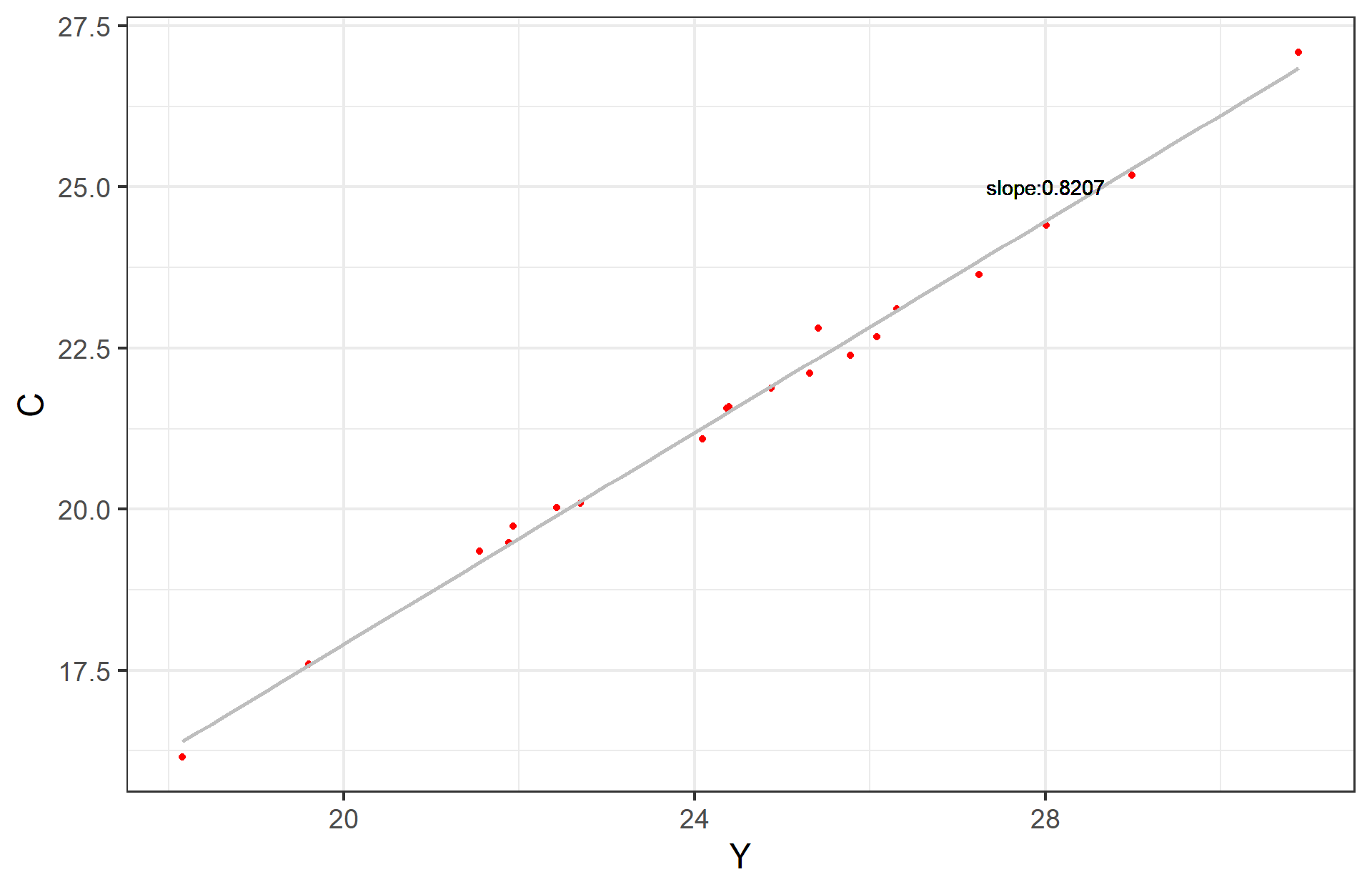
Manual calculation

According to the above formula, the regression coefficient can be calculated as follows:

Easy to calculate: \(\sum{u_ty_t}\) =3.8000

And: \(\sum{y^2_t}\) =184.0000

And: \(\frac{\sum{u_ty_t}}{\sum{y^2_t}}\) =0.0207

Hence： \(\hat{\beta}_1 = \beta_1 + \frac{\sum{u_ty_t}}{\sum{y^2_t}}\) =0.8+0.0207= 0.8207

This also means that \(\hat{\beta_1}\) is different from \(\beta_1=0.8\) , and the differnce is 0.0207.

According to the former provment procedure, we can manually calculate the OLS coefficient of beta_1.Finally, the OLS estimator of beta_1 equals 0.8207, and not equal to its true value 0.8 we have set before.So, the OLS estimator is biased with our simulation data set.

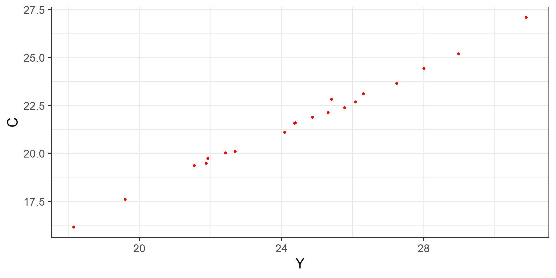
Scatter plots

Figure 5: The scatter of Y and C

Here, we draw the scatter of Y and C.

Regression report 1

Next, we used the simulated data for R analysis to obtain the original OLS report.

Call:
lm(formula = mod_monte$mod.C, data = monte)

Residuals:
     Min       1Q   Median       3Q      Max 
-0.27001 -0.15855 -0.00126  0.09268  0.46310 

Coefficients:
            Estimate Std. Error t value Pr(>|t|)    
(Intercept)  1.49402    0.35413   4.219 0.000516 ***
Y            0.82065    0.01434  57.209  < 2e-16 ***
---
Signif. codes:  0 '***' 0.001 '**' 0.01 '*' 0.05 '.' 0.1 ' ' 1

Residual standard error: 0.1946 on 18 degrees of freedom
Multiple R-squared:  0.9945,    Adjusted R-squared:  0.9942 
F-statistic:  3273 on 1 and 18 DF,  p-value: < 2.2e-16

Regression report 2

The tidy report of OLS estimation shows below.

\[ \begin{alignedat}{999} \begin{split} &\widehat{C}=&&+1.49&&+0.82Y_i\\ &(s)&&(0.3541)&&(0.0143)\\ &(t)&&(+4.22)&&(+57.21)\\ &(fit)&&R^2=0.9945&&\bar{R}^2=0.9942\\ &(Ftest)&&F^*=3272.87&&p=0.0000 \end{split} \end{alignedat} \]

\[ \begin{alignedat}{999} &\widehat{C}=&&+1.49&&+0.82Y\\ &\text{(t)}&&(4.2188)&&(57.2090)\\ &\text{(se)}&&(0.3541)&&(0.0143)\\ &\text{(fitness)}&& n=20;&& R^2=0.9945;&& \bar{R^2}=0.9942\\ & && F^{\ast}=3272.87;&& p=0.0000\\ \end{alignedat} \]

for sum, The results of direct use of OLS regression also show bias.

Sample regression line (SRL)

Figure 6: The SRL

And the OLS slope is 0.8207.

Conclusions and points

So let’s summarize this chapter.

• Compared with the single-equation model, the SEM involves more than one dependent or endogenous variable. So there must be as many equations as endogenous variables.

• SEM always show that the endogenous variables are correlated with stochastic terms in other equations.

• Classical OLS may not be appropriate because the estimators are inconsistent.

In the next chapter, we will learn the identification of SEM.See you in my next class. Goodbye.

Reference

• SimultaneousEq.pdf

End Of This Chapter