Table of chapter content

• Part 2：Simultaneous Equation Models (SEM)
• Chapter 17. Endogeneity and Instumental Variables
• 17.1 Definition and sources of endogeneity
• 17.2 Estimation problem with endogeneity
• 17.3 IV and the choices
• 17.4 Two-stage least squares method
• 17.5 Testing Instrument validity
• 17.6 Testing Regressor endogeneity
• chapter Summary
• Exercise and Computation

Advanced Econometrics III

(Econometrics III)

Chapter 17. Endogeneity and Instumental Variables

Hu Huaping (胡华平)

huhuaping01 at hotmail.com

School of Economics and Management (经济管理学院)

2025-04-19

Good evening everyone. Welcome to my class.I am teacher Hu Huaping.Here is my email.You can contact me when you have any questions with our course.In this part, we will learn Simultaneous Equation Models together by using almost eight lessons.

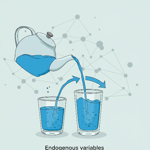
Part 2：Simultaneous Equation Models (SEM)

Chapter 17. Endogeneity and Instrumental Variables

Chapter 18. Why Should We Concern SEM ?

Chapter 19. What is the Identification Problem ?

Chapter 20. How to Estimate SEM ?

As you see this part contains four chapters.Firstly, we will go through Chapter 17. Regressor Endogeneity problems and instrumental Variables solutions will be discussed in this chapter. Anyway, this chapter will be a good start for learning SEM.The next three chapters focus closely on SEM. We will answer three important questions in turn.In Chapter 18, we will know SEM is important in social science and it also brings new challenges to us.Large SEM system always contains lots of parameters need to be solved and will face with the identification problems. We will give you guides and rules to check the SEM identification status in Chapter 19.Finally, we will discuss different SEM estimation approaches in Chapter 20, including 2SLS, Three-stage least squares (3SLS) and full information maximum likelihood (FIML) method.

Chapter 17. Endogeneity and Instumental Variables

17.1 Definition and source of endogeneity

17.2 Estimation problem with endogeneity

17.3 IV and choices

17.4 Two-stage least squares method

17.5 Testing instrument validity

17.6 Testing regressor endogeneity

sourceSo let us start the first chapter.In this chapter:- You will see how the method of instrumental variables (IV) can be used to solve the problem of endogeneity due to one or more regressors.- Also we will learn the method of two stage least squares in section 17.4. 2SLS method is second in popularity only to ordinary least squares for estimating linear equations in econometrics.- And some useful testing techniques will be introduced to check instrument validity and regressor endogeneity. These content will be uncovered in the last two sections.

17.1 Definition and sources of endogeneity

In this section we will talk about the definition of endogeneity and its main sources.The story begins with the stochastic regressors.

Review

CLRM Assumptions and Random Experiments

这张图展示了经典线性回归模型(CLRM)的关键假设和随机试验的概念。左侧列出了CLRM的五个基本假设,右侧说明了随机试验的特点。这有助于学生回顾之前学习的重要概念。

The CLRM assumptions

Let’s revise the classic linear regression model assumptions (CLRM):

• A1: The true model is \(\boldsymbol{y= X \beta+\epsilon}\).

• A2: \(\forall i, E(\epsilon_i|X) = 0\) (conditional zero mean) more about this later.

• A3: \(Var(\epsilon|X) = E(\epsilon \epsilon^{\prime}|X) = \sigma^2I\) (identical conditional variance ).

• A4: \(\boldsymbol{X}\) has full column rank.

• A5: (for inference purposes,\(\boldsymbol{\epsilon} \sim N(\boldsymbol{0}, σ^2\boldsymbol{I}))\).

Under A1-A4（also namely CLRM）, the OLS is Gauss-Markov efficient.

Under A1-A5, we donote N-CLRM.

we have discussed these assumptions before the class. And we denote the Gauss-Markov model assumption system as classical linear regression model (CLRM).- Assumption 1: The model is assumed to be true and be linear with parameters.- Assumption 2: the disturbance term has conditional zero expectation. And we will relax this assumption later.- Assumption 3: this means the conditional variance of disturcances is identity given X. the other way to express assumption 3 is that the disturbance term is homoscedasticity[’hɔməusi,dæs’tisəti].- Assumption 4: The regressor matrix X has full column rank. Which means that none of the regressors is the perfect linear function on the rest of the regressors.- Assumption 5: We will bring in the norm distribution assumption on the disburtance. This assumption aims for hypothesis testing purposes.Joint with A2, A3, and A5, the disturbance is assumed to be normally identical independent distribution. We just write i.i.d for shortly.With assumptions A1-A4, We note CLRM. Under CLRM the OLS is Gauss-Markov efficient. Which means under CLRM, when we use OLS method we will obtain the Best-Linear-unbiased estimators on the true parameters. [hand writing]While, with assumptions A1-A5, we used to denote as N-CLRM. we can conduct kinds of inference and tests based on N-CLRM.Now let us focus on assumption 2.

The A2 assumptions

For the population regression model(PRM):

\[ \begin{align} Y_i &= \beta_1 +\beta_2X_i + u_i && \text{(PRM)} \end{align} \]

• CLRM A2 assumes that \(X\) is fixed (given) or independent of the error term. The regressors \(X\) are not random variables. At this point, we can use the OLS method and get BLUE (Best Linear Unbiased Estimator).

\[ \begin{align} Cov(X_i, u_i)= 0; \quad E(X_i u_i)= 0 \end{align} \]

• If the above A2 assumption is violated, the independent variable \(X\) is related to the random disturbance term. In this case, OLS estimation will no longer get BLUE, and instrumental variable method (IV) should be used for estimation.

\[ \begin{align} Cov(X_i, u_i) \neq 0 ; \quad E(X_i u_i) \neq 0 \end{align} \]

If A2 is violated, then the endogeneity problem arise.Now we go head to define the endogenous variable.事实上，无论\(X_i\)与\(u_i\)是否相关，我们都可以采用IV法得到BLUE。

Good model & Random experiment

Randomized controlled experiment : Ideally, the value of the independent variable \(X\) is randomly changed (refer to the reason), and then we look at the change in the dependent variable \(Y\) (refer to the result).

\[ \begin{equation} \boldsymbol{y= X \beta+u} \end{equation} \]

• If \(Y_i\) and \(X_i\) does exist systematic relationship (linear relationship), then change \(X_i\) causes the corresponding change of \(Y_i\).

• Any other random factors will be added to the random disturbance \(u_i\). The effect of the random disturbance on the change of \(Y_i\) should be independent to the effect of \(X_i\) on the change of \(Y_i\).

Exogenous regressors

Exogenous regressors: If independent variables \(X_i\) is perfectly random (randomly assigned) as mentioned above , then they are called exogenous regressor. More precisely, they can be defined as:

Strictly Exogeneity：

\[ E\left(u_{i} \mid X_{1}, \ldots, X_{N}\right)=E\left(u_{i} \mid \mathbf{x}\right)=0 \]

因为在随机控制实验，给定样本\(i\)和样本\(j\)，自变量的取值分别为 \(X_i\)和\(X_j\)，它们应该是相互独立的。因此可以把上述假设进一步简化为：> 同期外生性假设（contemporaneously exogeneity）：\(E(u_i|X_{i})=0, \text{for } i =1, \ldots,N\)。同期表示的是在同样的时间点上，或所有的截面观测单位在某个时间上获得的观测。大样本情况下OLS方法在大样本情形下，上述严格外生性假设可以进一步转换为同期不相关假设：- \(E(u_i)=0\)，而且- \(\operatorname{cov}(X_i, u_i)=0\)因为我们可以证明（证明略），在大样本情况OLS方法下：- \(E(u_i|X_{i})=0 \quad \Rightarrow \quad E(u_i)=0\)- \(E(u_i|X_{i})=0 \quad \Rightarrow \quad \operatorname{cov}(X_i, u_i)=0\)

Endogeneity

Definition of endogeneity

The concept of endogeneity is used broadly to describe any situation where a regressor is correlated with the error term.

• Assume that we have the bivariate linear model

\[ \begin{equation} Y_{i}=\beta_{0}+\beta_{1} X_{i}+\epsilon_{i} \end{equation} \]

• The explanatory variable \(X\) is said to be Endogenous if it is correlated with \(\epsilon\).

\[ \begin{align} Cov(X_i, \epsilon_i) \neq 0 ; \quad E(X_i \epsilon_i) \neq 0 \end{align} \]

• And if \(X\) is uncorrelated with\(\epsilon\), it is said to be Exogenous.

\[ \begin{align} Cov(X_i, \epsilon_i) = 0 ; \quad E(X_i \epsilon_i) = 0 \end{align} \]

We use the term endogeneity frequently in econometrics.

Next, we should ask what the sources of endogeneity come from.

Sources of endogeneity

In applied econometrics, endogeneity usually arises in one of four ways:

• Omitted variables: when the model is set incorrectly.

• Measurement errors in the regressors.

• Autocorrelation of the error term in autoregressive models.

• Simultaneity: when \(\boldsymbol{Y}\) and \(\boldsymbol{X}\) are simultaneously determined, as in the supply/demand model (we will go to explain it in the next three chapter).

So, let us go through all of these four situations quickly.

Source 1: Omitted variables

生图提示词：

I am a university teacher. I want to generate a picture on the concept of endogeneity on my econometrics class to my students. the picture should be: Simple line drawing style, transparent background. On the left side draw a diploma icon (education variable), right side a money bag (wage). Draw solid arrow from diploma to money bag labeled ‘Estimated effect’. Above them draw a brain icon (ability variable) sending dashed arrows to both diploma and money bag, with red cross over the brain. Add warning sign at bottom with text ‘Omitted Variable Causes Endogeneity’. All elements in black lines, minimalist academic diagram style.

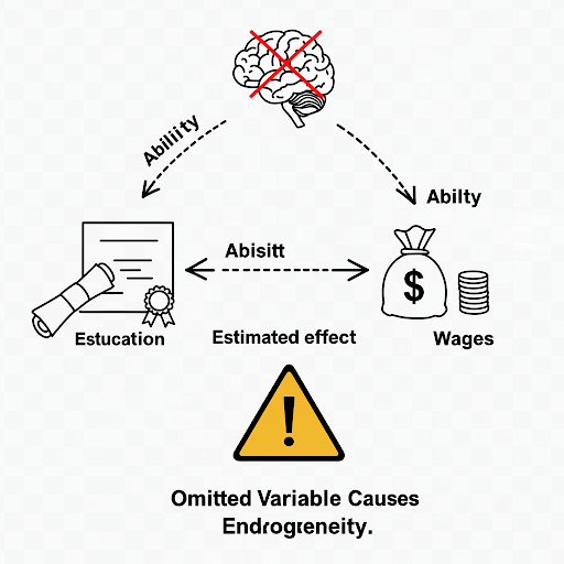
The assumed true model & mis-specified model

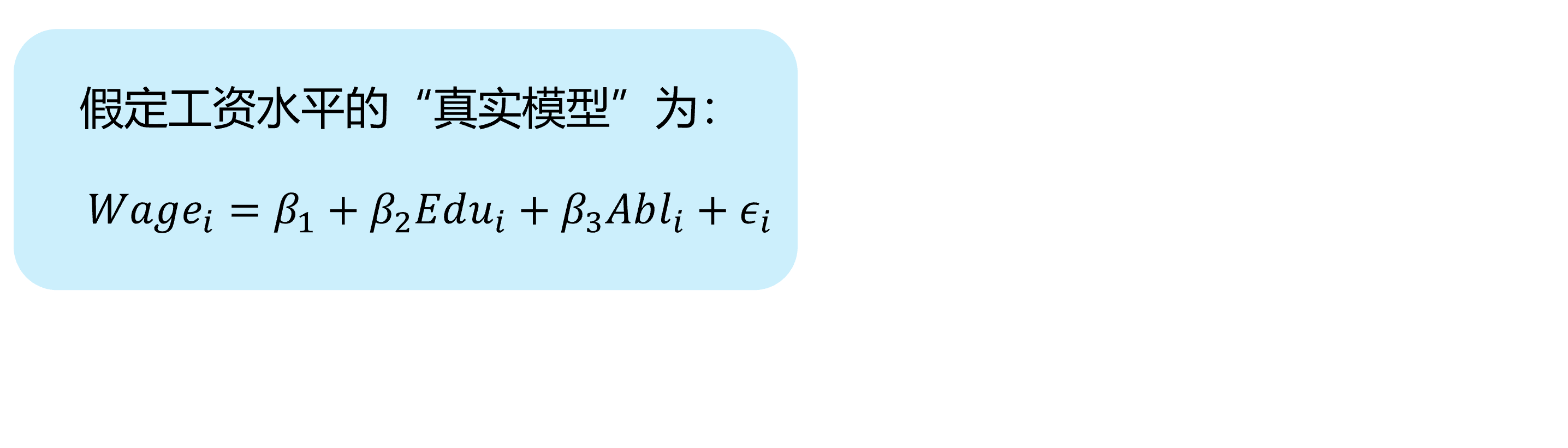
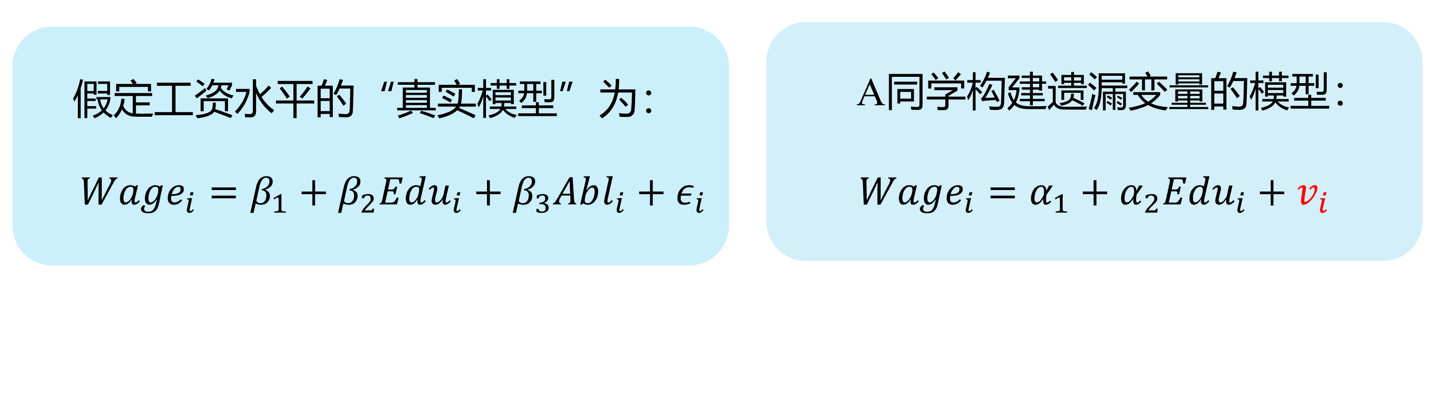
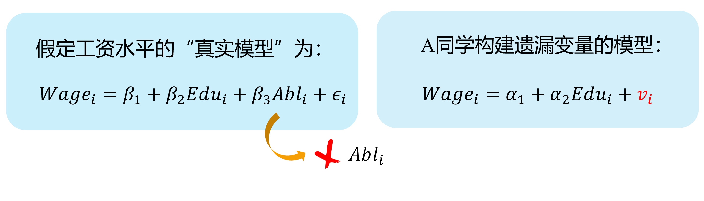
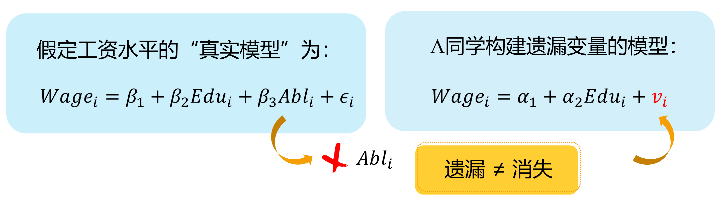
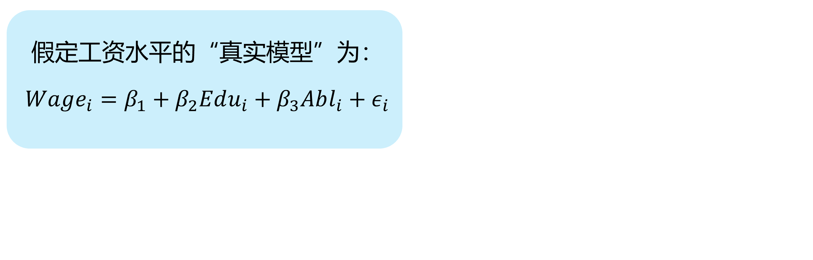
Suppose that the “assumed true model” for wage determination is:

\[ \begin{align} Wage_{i}=\beta_{1}+\beta_{2} Edu_{i}+\beta_{3} Abl_{i}+\epsilon_{i} \quad \text{(the assumed true model)} \end{align} \]

However, because the individual’s ability variable (\(Abl\)) is often not directly observed, so we often can’t put it into the model, and build a mis-specified model.

\[ \begin{align} Wage_{i}=\alpha_{1}+\alpha_{2} Edu_{i}+v_{i} \quad \text{(the mis-specified model)} \end{align} \]

• Where ability variable (\(Abl\)) is included in the new disturbance \(v_i\), and \(v_{i}=\beta_{3} abl_{i}+u_{i}\)

• Obviously, in the mis-specified model, we ignore the ability variable (\(Abl\)), while variable years of education (\(Edu\)) is actually related to it.

• So in the mis-specified model, \(cov(Edu_i, v_i) \neq 0\), thus years of education (\(Edu\)) may cause the endogenous problem.

why the variables are Omitted? Because people run a model without considering the necessary or important variables we should.We will explain later that Omission of relevant variable will result in inconsistent estimates because A2 is not hold.Now, let us talk about the second source of endogeneity. the Measurement error in the regressors.

Omitted variables (demo 1/4)

Here we show a visual demonstration on this situation:

Assumed “TRUE MODEL”:

Omitted variables (demo 2/4)

Here we show a visual demonstration on this situation:

Assumed “TRUE MODEL”:

“A’s mis-specification MODEL”:

Omitted variables (demo 3/4)

Here we show a visual demonstration on this situation:

Assumed “TRUE MODEL”:

“A’s mis-specification MODEL”:

Omitted variables (demo 4/4)

Here we show a visual demonstration on this situation:

Assumed “TRUE MODEL”:

“A’s mis-specification MODEL”:

Omitted\(\neq\) Disappeared

Source 2: Measurement errors

test show

The assumed true model & mis-specified model

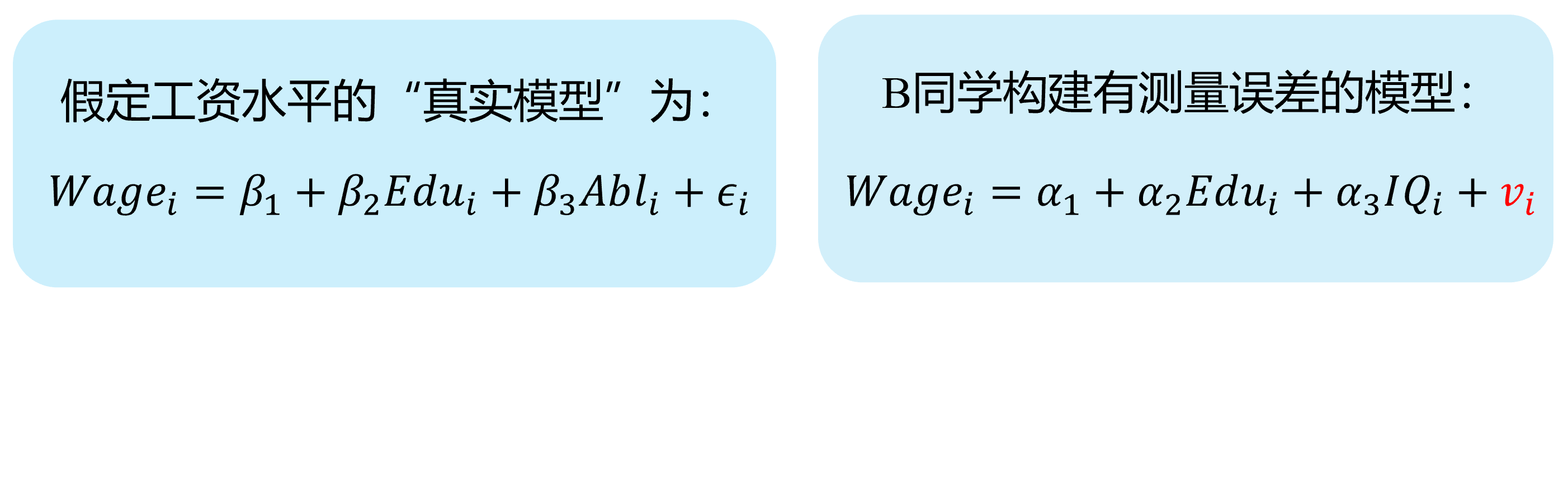
Again, let’s consider the “assumed true model”:

\[ \begin{align} Wage_{i}=\beta_{1}+\beta_{2} Edu_{i}+\beta_{3} Abl_{i}+\epsilon_{i} \quad \text{(the assumed true model)} \end{align} \]

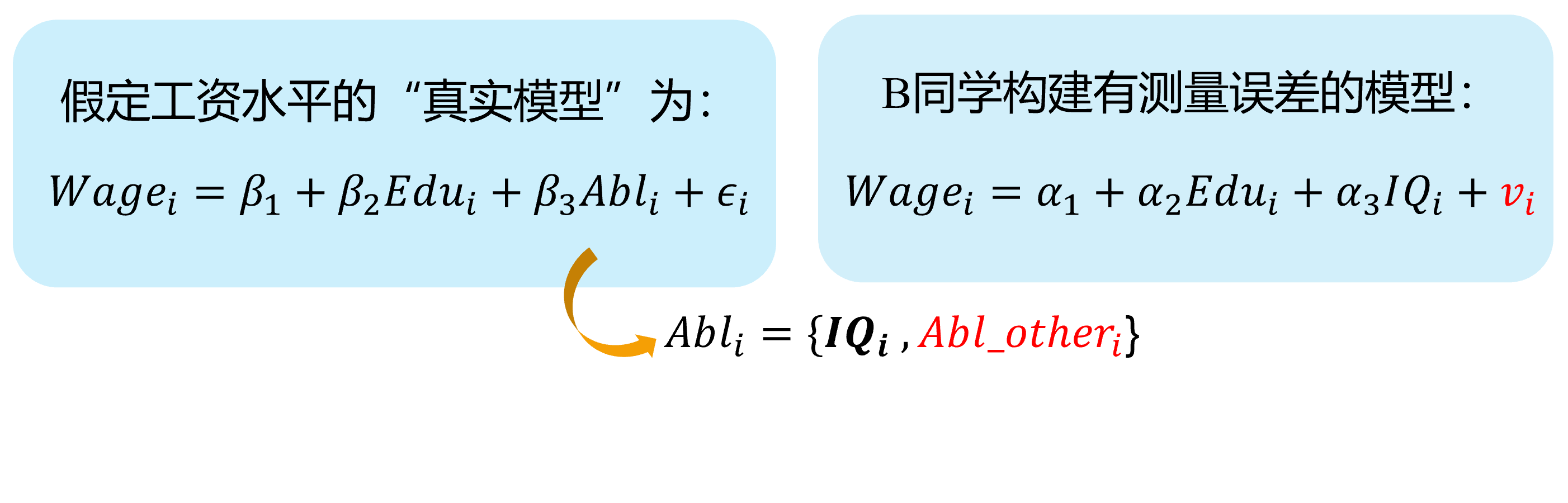
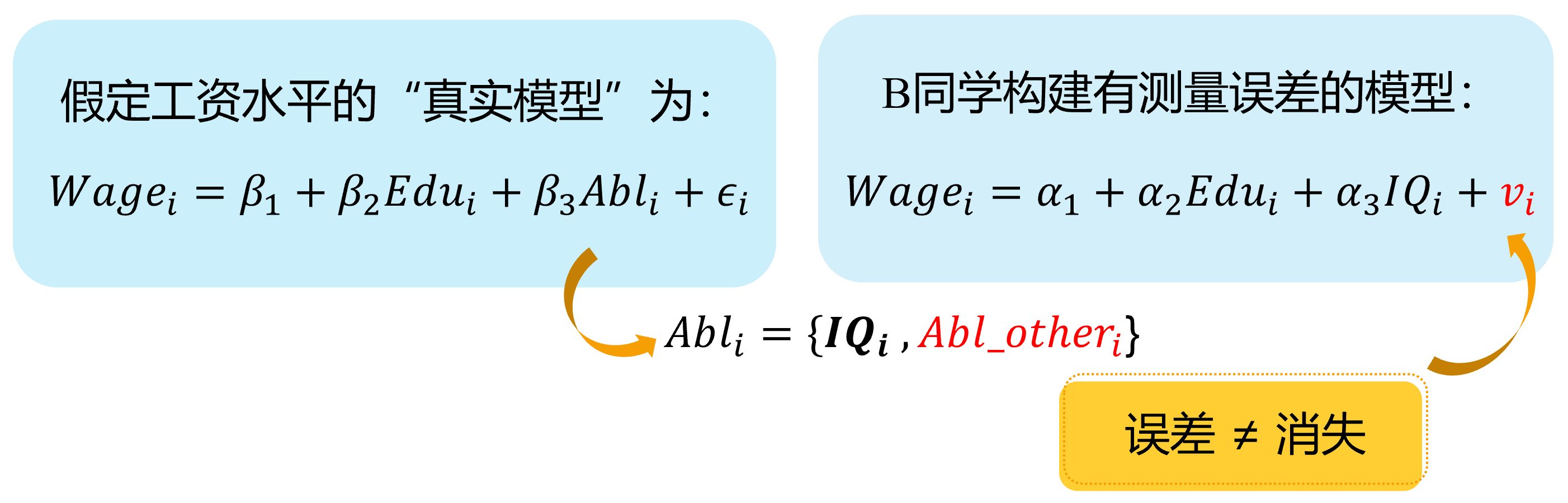
It is hard to observe individual’s ability variable(\(Abl\)), and somebody will instead to use the variable IQ score(\(IQ_i\)), and construct the mis-specified “proxy variable” model:

\[ \begin {align} Wage_i=\alpha_{1}+\alpha_{2} Edu_i+\alpha_{3} IQ_i+v_i \quad \text{(the mis-specified model)} \end {align} \]

• It should exist stuffs (\(Abl\_other_i\)) which the model does not include (due to the measurement error). So the measurement errors (\(Abl\_other_i\)) will go to the disturbance term\(v_i\) in the mis-specified model.

• And we know that measurement errors (\(Abl\_other_i\)) will be correlated with the education variable. Thus \(cov(Edu_i, v_i) \neq 0\), and the education variable(\(Edu\)) may cause the endogenouse problem.

In practice, the observation value of a regressor is not accurate, in most time is only the “approximation”.So there is measurement error in the regressor in our model.

Measurement errors (demo 1/4)

Here we show a visual demonstration on this situation:

Assumed TRUE MODEL:

Measurement errors (demo 2/4)

Here we show a visual demonstration on this situation:

Assumed TRUE MODEL:

B’s mis-specification MODEL:

Measurement errors (demo 3/4)

Here we show a visual demonstration on this situation:

Assumed TRUE MODEL:

B’s mis-specification MODEL:

Measurement errors (demo 4/4)

Here we show a visual demonstration on this situation:

Assumed TRUE MODEL:

B’s mis-specification MODEL:

Measure Error\(\neq\) Disappeared

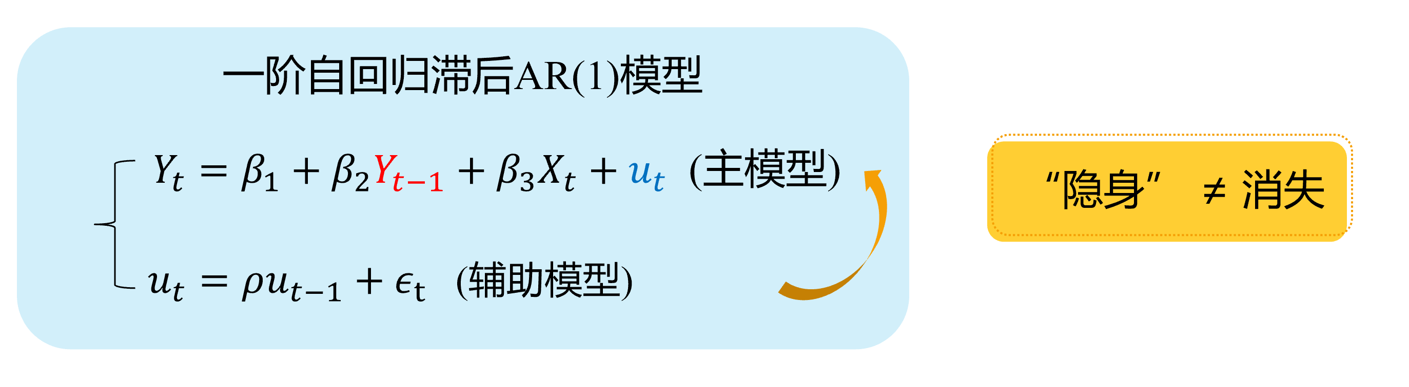
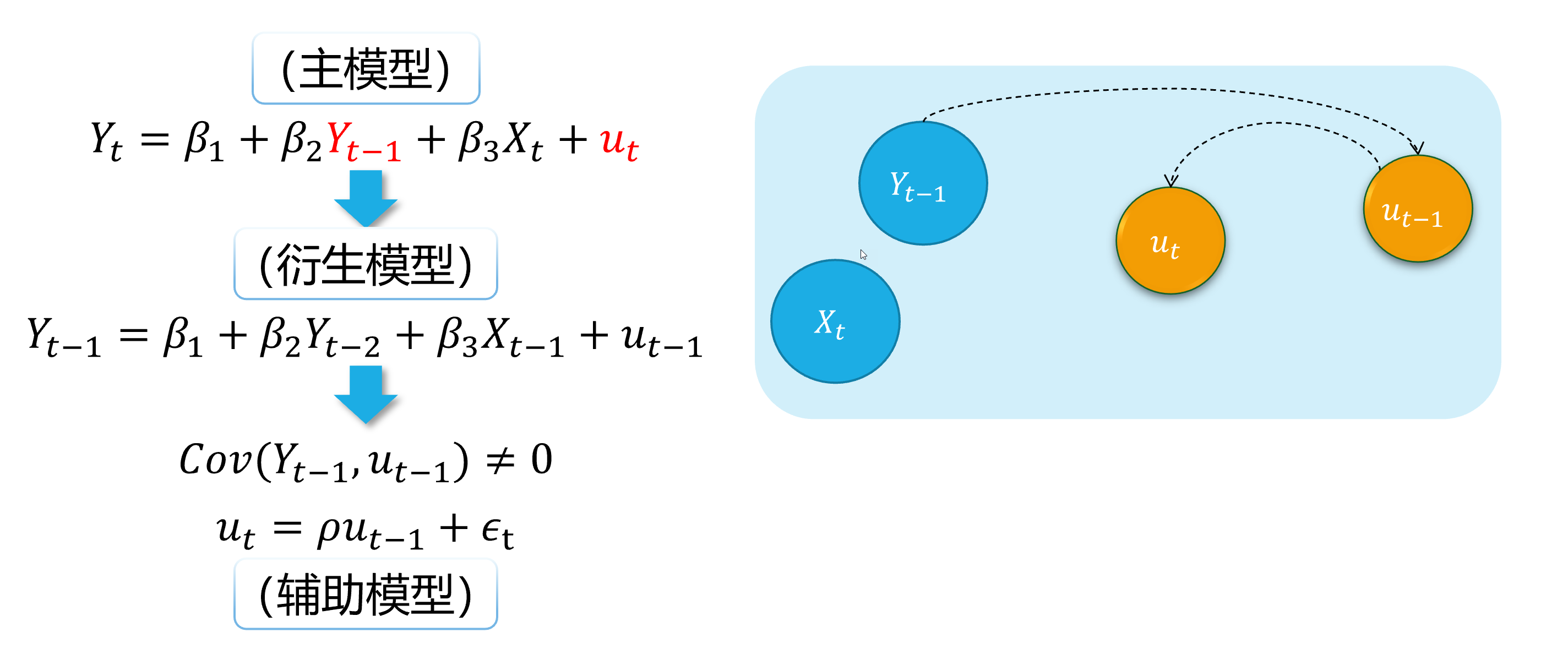
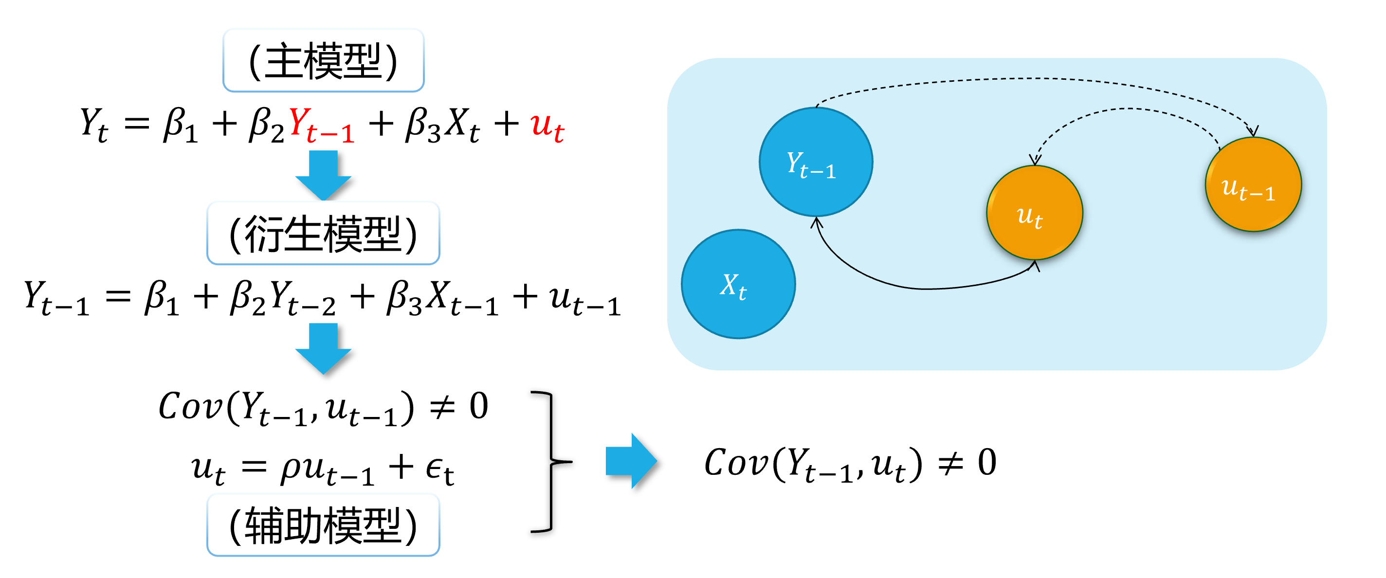
Source 3: Autocorrelation

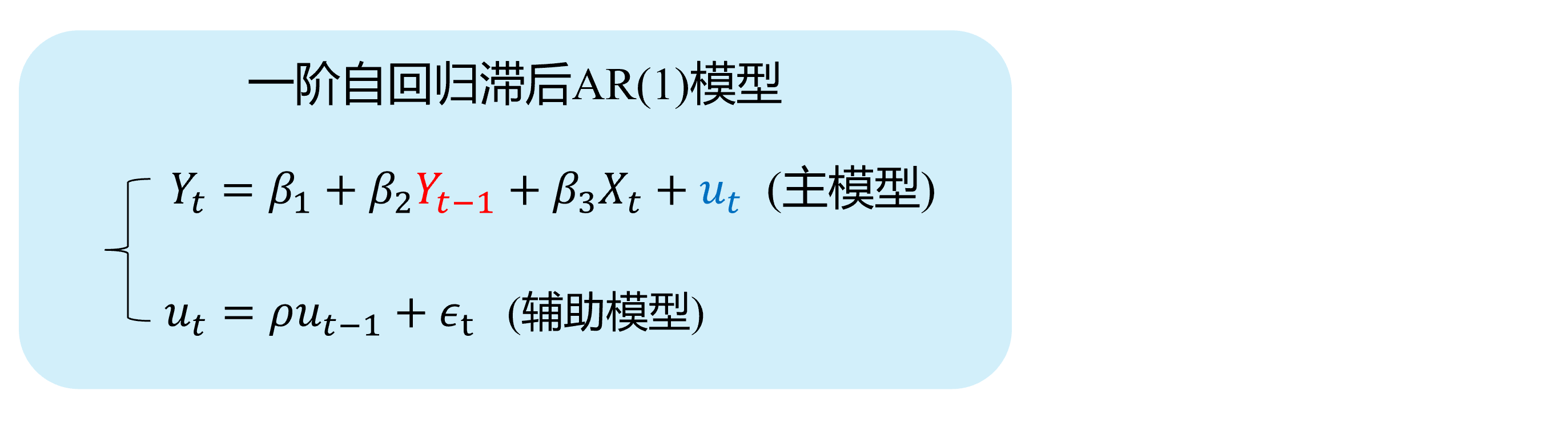
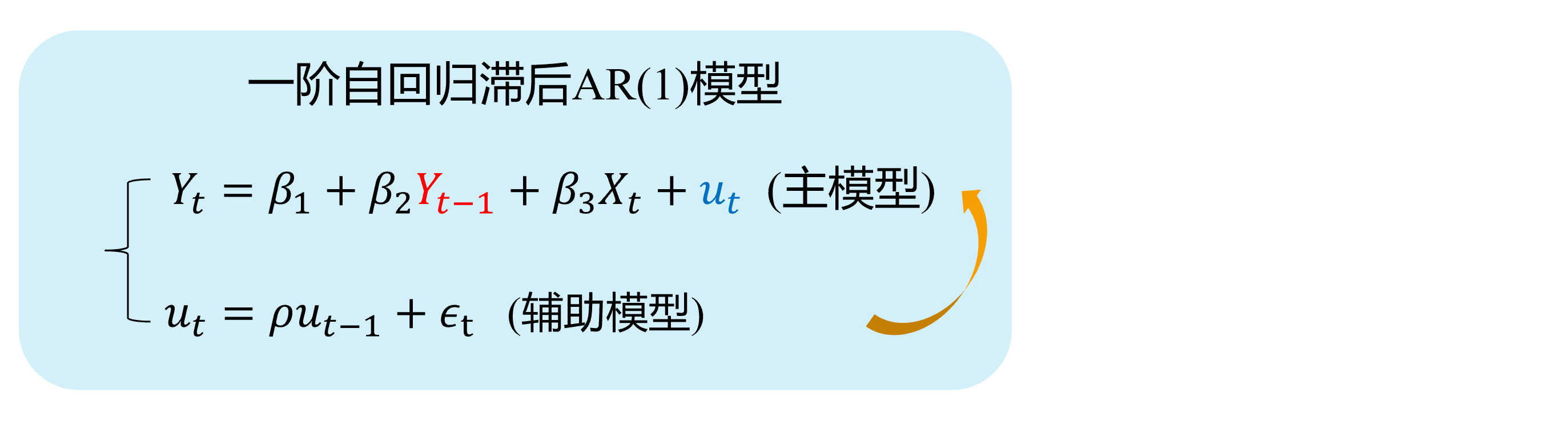
The autoregressive model with AR(1)

Autoregressive model: Lag variable of dependent variable(\(Y_{t-1}, \ldots, Y_{t-p},\ldots\)) appears in the model as regressors.

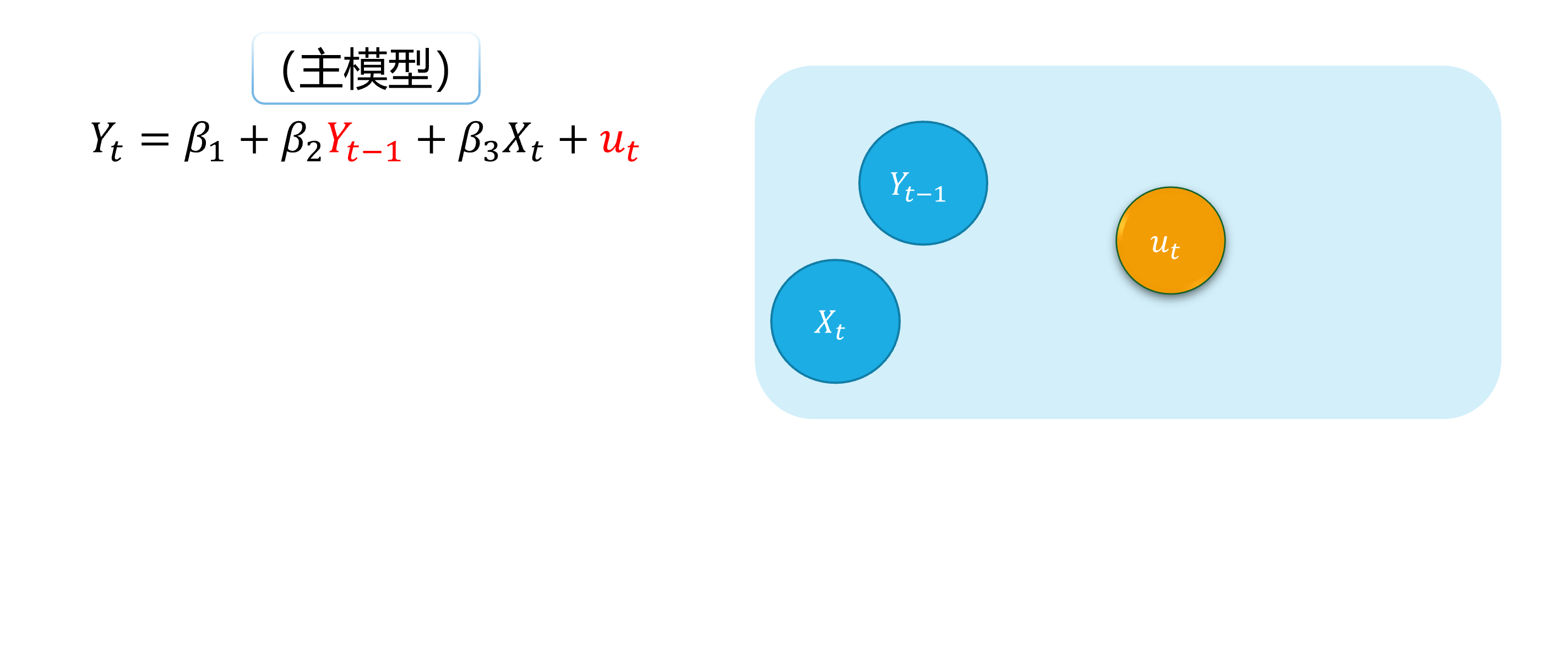
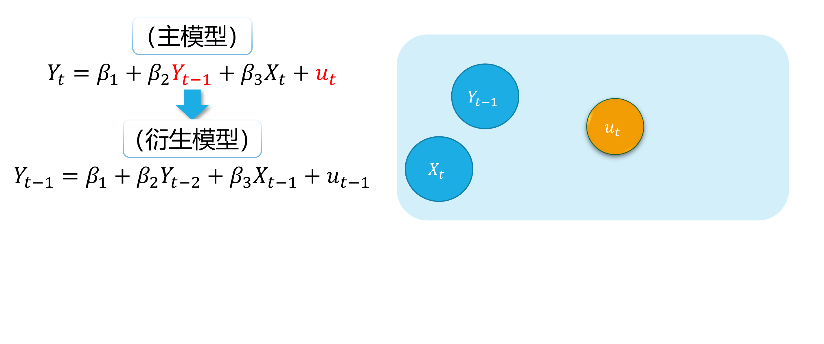
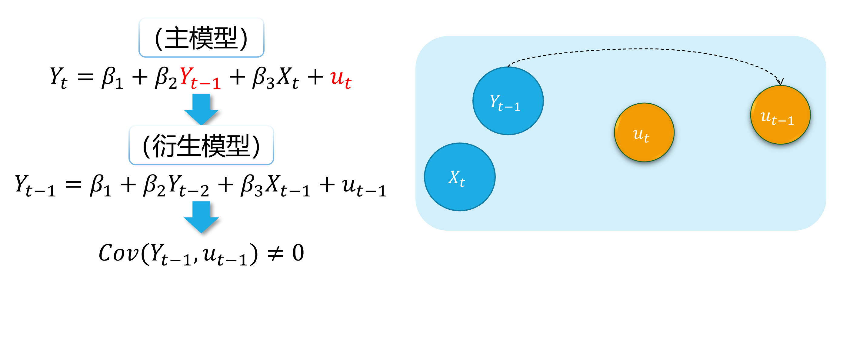
\[ \begin {align} Y_t=\beta_{1}+\beta_{2} Y_{t-1}+\beta_{3}X_t+u_t \end {align} \]

If the disturbance term determined following a first-order autocorrelation AR(1):

\[ \begin {align} u_t=\rho u_{t-1}+ \epsilon_t \end {align} \]

Then, it is obvious that \(cov(Y_{t-1}, u_{t-1}) \neq 0\) and \(cov(Y_{t-1}, u_{t}) \neq 0\).

Thus the lag dependent variable (\(Y_{t-1}\)) will cause the endogeneity problem in the Autoregressive model.

Autocorrelation (demo 1) 1/4

Here we show a visual demonstration on this situation:

Assumed TRUE MODEL: AR(1)

Autocorrelation (demo 1)2/4

Here we show a visual demonstration on this situation:

Assumed TRUE MODEL: AR(1)

(main model)

(auxiliary model)

Autocorrelation (demo 1)3/4

Here we show a visual demonstration on this situation:

Assumed TRUE MODEL: AR(1)

(main model)

(auxiliary model)

Autocorrelation (demo 1) 4/4

Here we show a visual demonstration on this situation:

Assumed TRUE MODEL: AR(1)

(main model)

(auxiliary model)

Hidden\(\neq\) Disappeared

Autocorrelation (demo 2) 1/5

An intuitive demonstration is show as follows:

(main model)

Autocorrelation (demo 2) 2/5

An intuitive demonstration is show as follows:

(main model)

(derived model)

Autocorrelation (demo 2) 3/5

An intuitive demonstration is show as follows:

(main model)

(derived model)

Autocorrelation (demo 4) 1/5

An intuitive demonstration is show as follows:

(main model)

(derived model)

(auxiliary model)

Autocorrelation (demo 2) 5/5

An intuitive demonstration is show as follows:

(main model)

(derived model)

(auxiliary model)

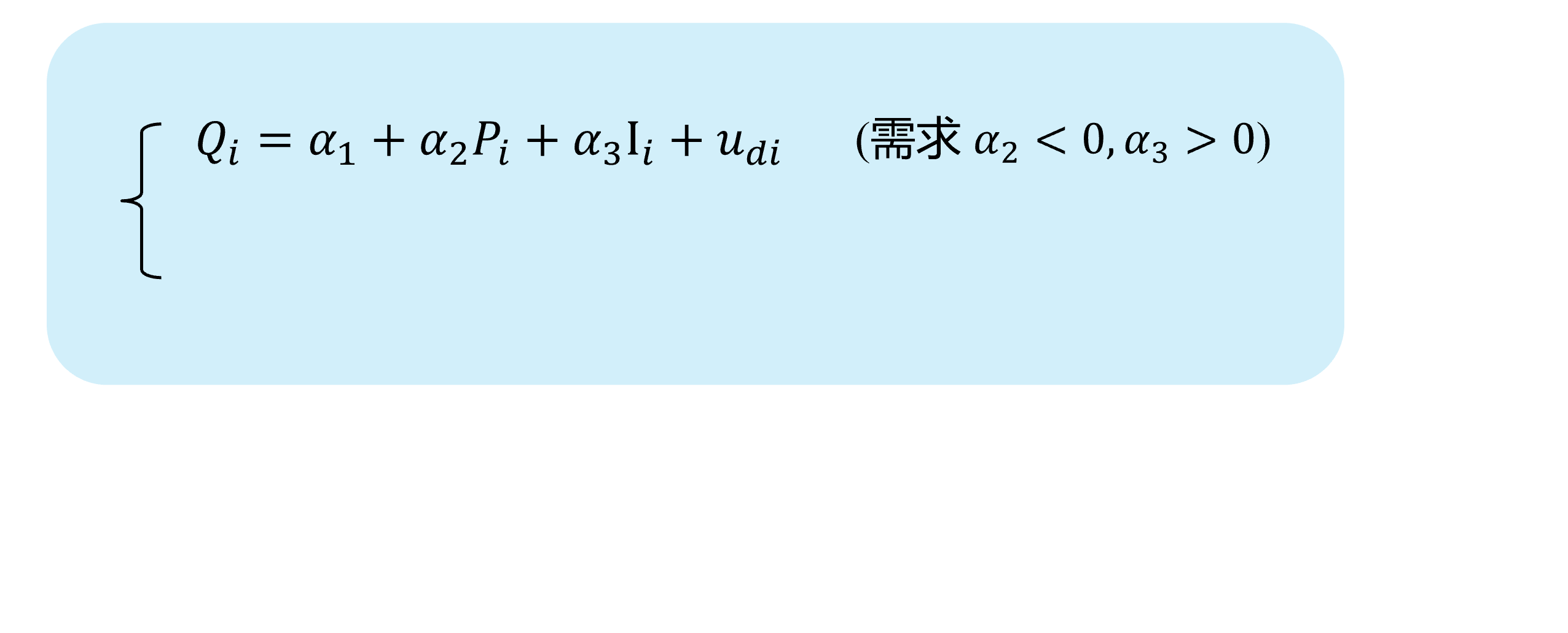
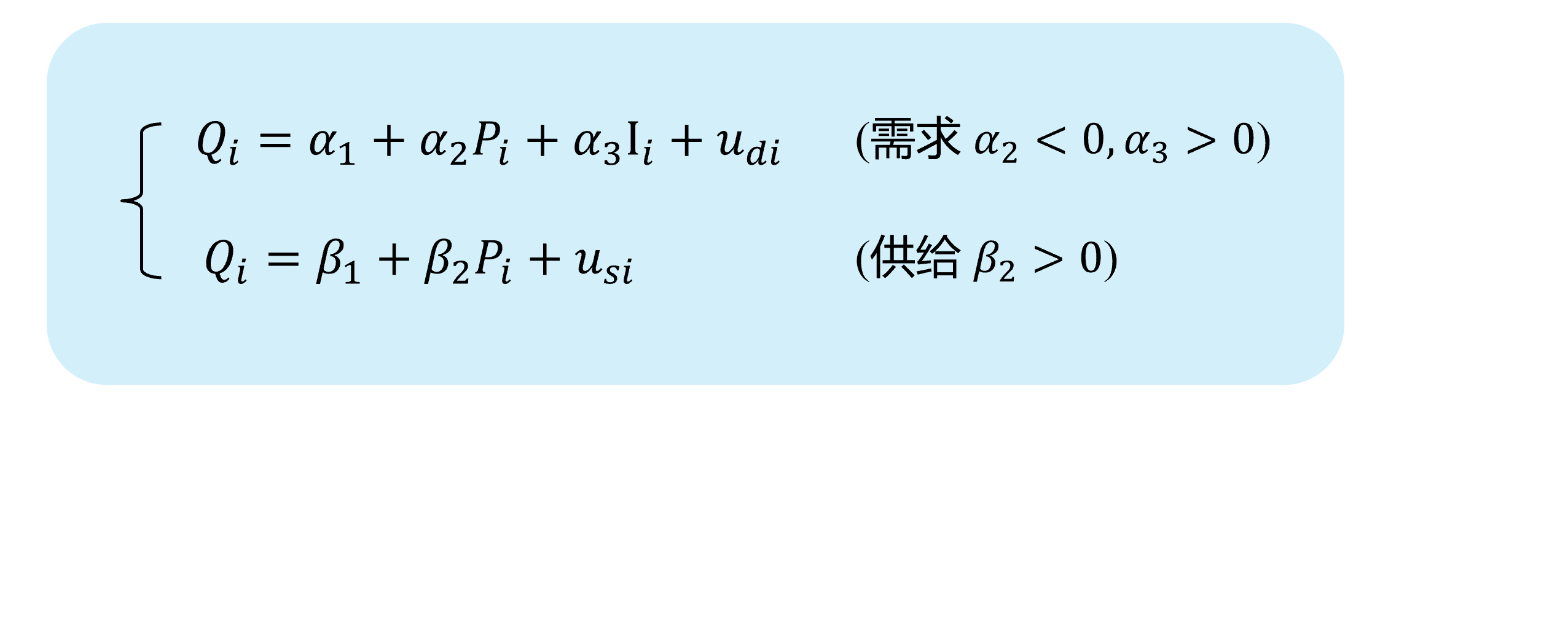
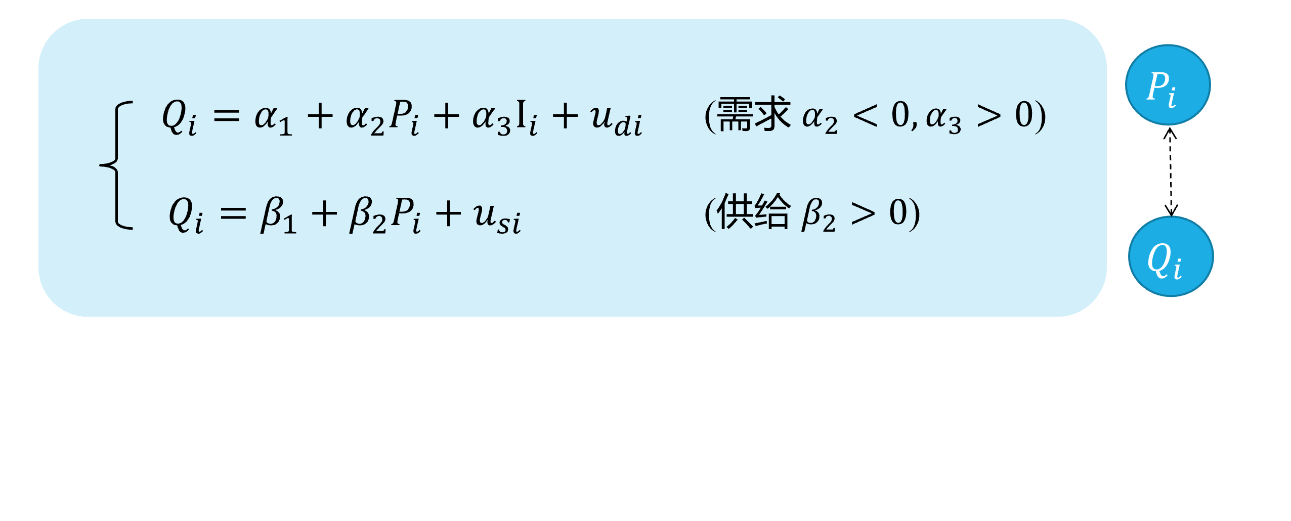
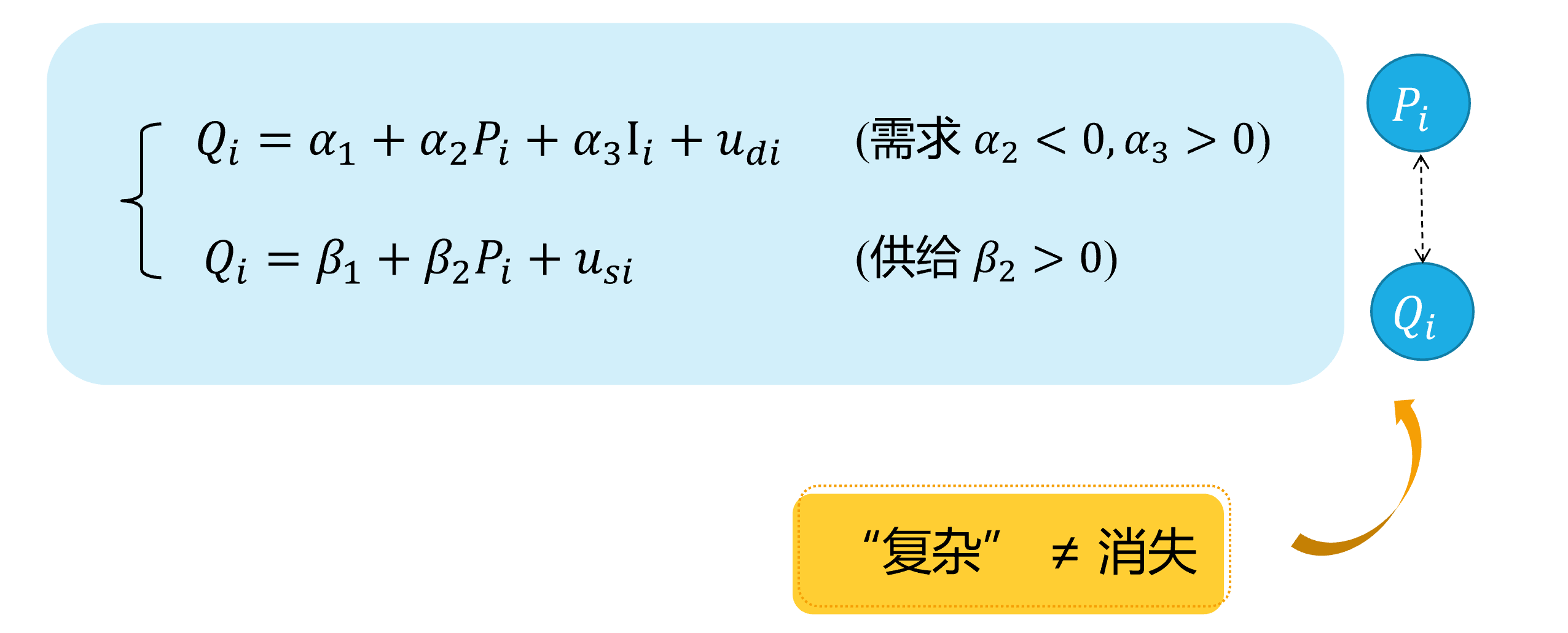
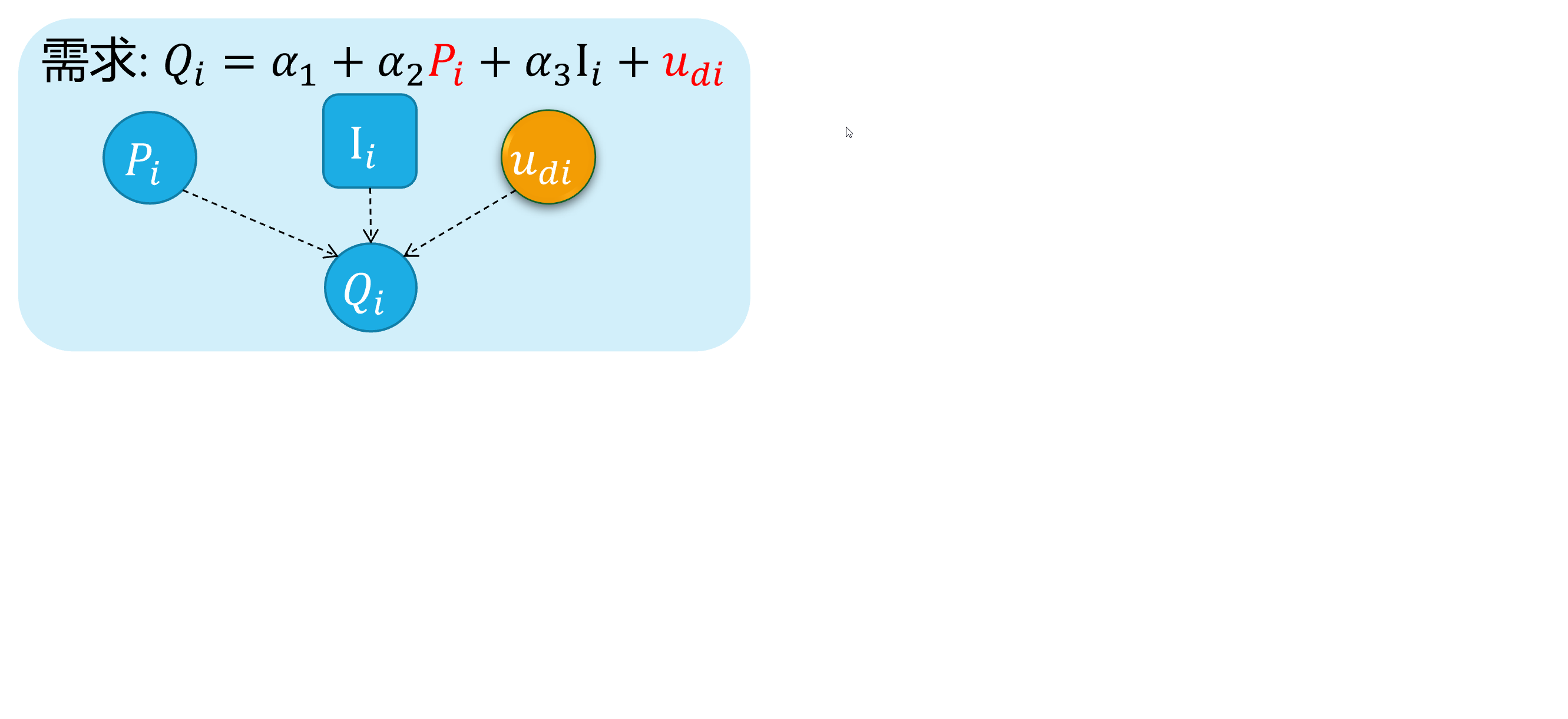
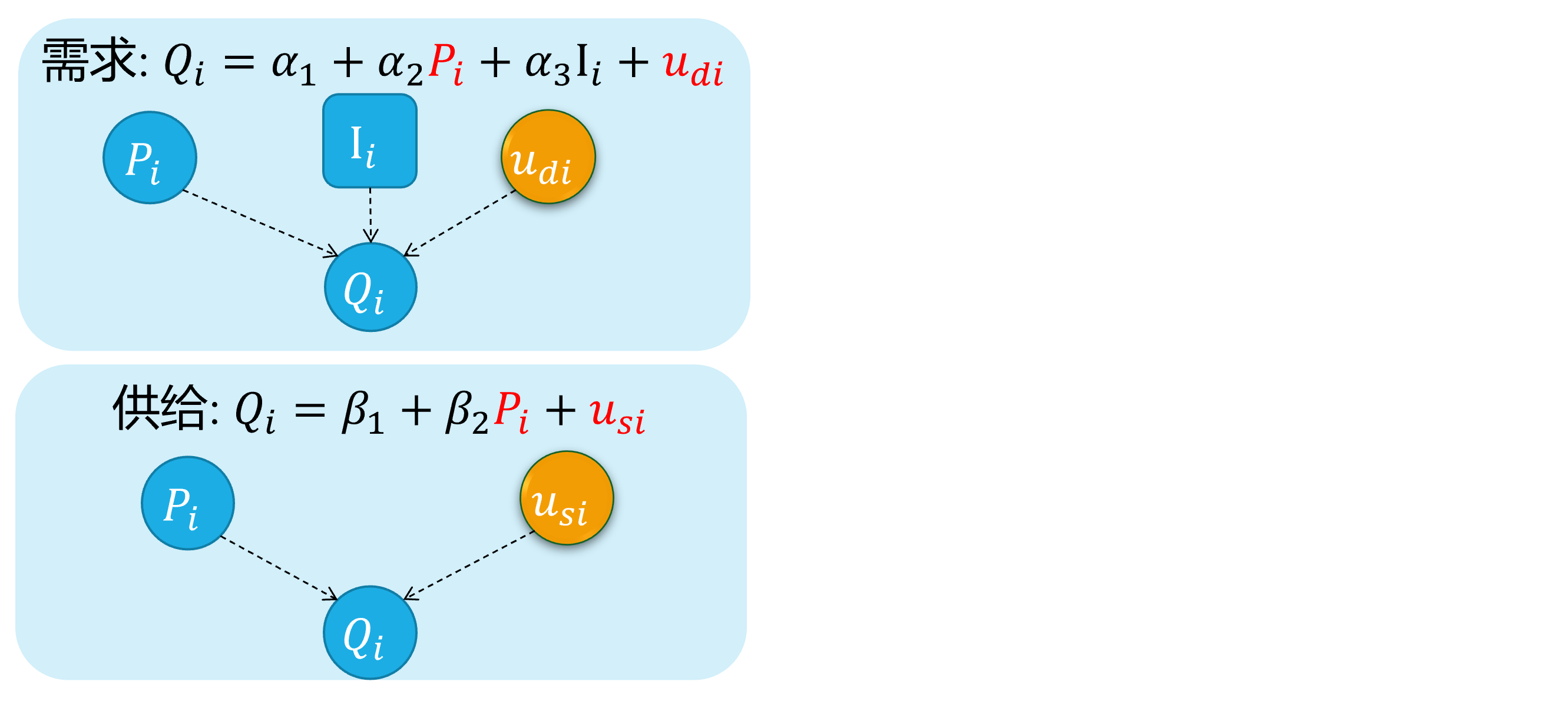
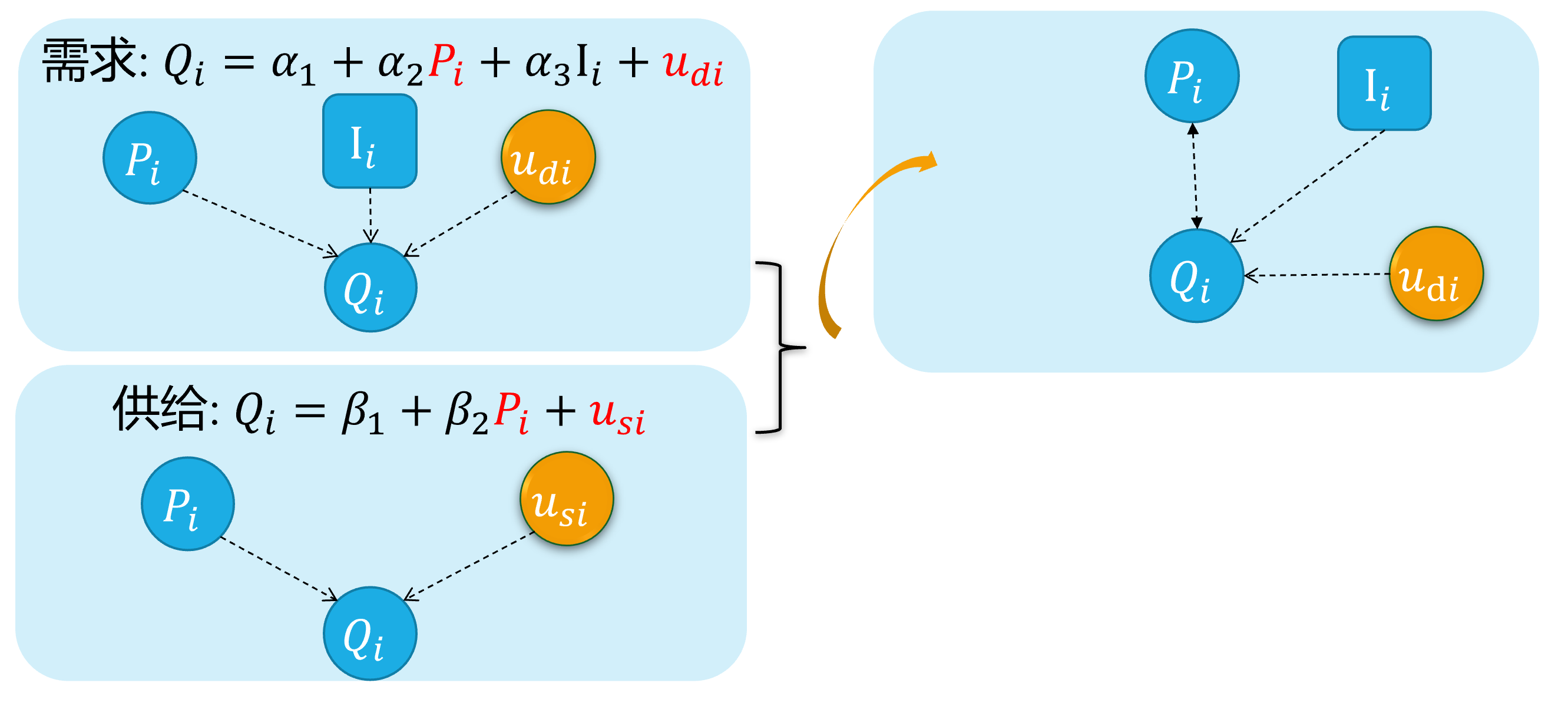
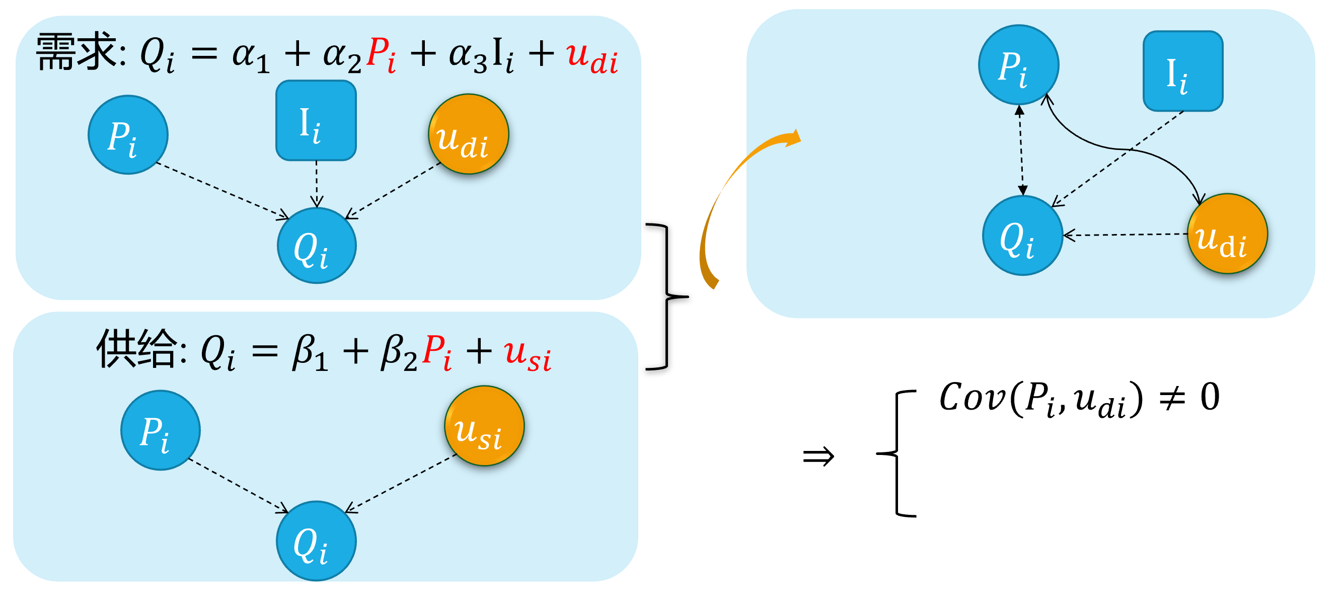
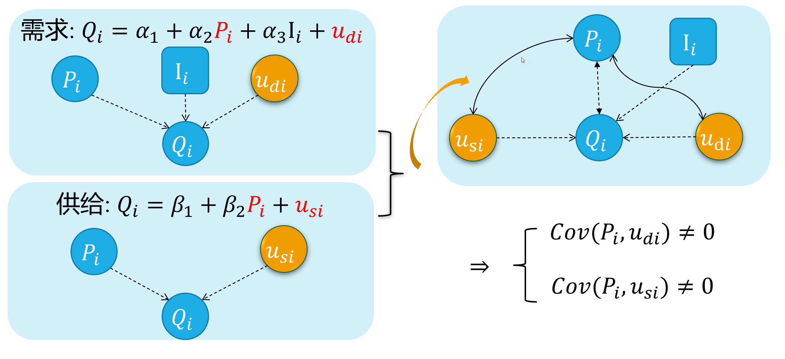
Source 4: Simultaneity

The simultaneous equation model system

For the equations system of supply and demand:

\[ \begin{cases} \begin{align} \text { Demand: } & Q_{i}=\alpha_{1}+\alpha_{2} P_{i}+u_{d i} \\ \text { Supply: } & Q_{i}=\beta_{1}+\beta_{2} P_{i} + u_{s i} \end{align} \end{cases} \]

As we all know, because of the price \(P_i\) will both affect supply and the demand \(Q_i\), And vice versa. There is a feedback cycle mechanism in this system.

So, we can get \(cov(P_i, u_{di}) \neq 0\), and \(cov(P_i, u_{si}) \neq 0\), which will cause the endogenous problem finally.

/ˌsɪmltəˈneɪət/

Simultaneity (demo 1) 1/4

Here we show a visual demonstration on this situation:

(Demand

Simultaneity (demo 1) 2/4

Here we show a visual demonstration on this situation:

(Demand

(Supply

Simultaneity (demo 1) 3/4

Here we show a visual demonstration on this situation:

(Demand

(Supply

Simultaneity (demo 1) 4/4

Here we show a visual demonstration on this situation:

(Demand

(Supply

Hidden\(\neq\) Disappeared

Simultaneity (demo 2) 1/5

An intuitive demonstration is show as follows:

D:

Simultaneity (demo 2) 2/5

An intuitive demonstration is show as follows:

D:

S:

Simultaneity (demo 2) 3/5

An intuitive demonstration is show as follows:

D:

S:

Simultaneity (demo 2) 4/5

An intuitive demonstration is show as follows:

D:

S:

Simultaneity (demo 2) 5/5

An intuitive demonstration is show as follows:

D:

S:

17.2 Estimation problem with endogeneity

The question is what will happen on OLS estimators with model contains endogenous regressors.So, let us illustrate these estimation problems in detail in this section.we will discuss along two different situations.

Inconsistent estimates

mis-specified model with measurement error

Consider the simple regression model:

\[ \begin{align} Y_{i}=\beta_{0}+\beta_{1} X_{i}+\epsilon_{i} \quad \text{(1)} \end{align} \]

We would like to measure the effect of the variable\(X\) on\(Y\), but we can observe only an imperfect measure of it (i.e. a proxy variable), which is

\[ \begin{align} X^{\ast}_{i}=X_{i} - v_{i} \quad \text{(2)} \end{align} \]

Where\(v_i\) is a random disturbance with mean 0 and variance\(\sigma_{v}^{2}\).

Further, let’s assume that\(X_i, \epsilon_i\) and\(v_i\) are pairwise independent.

In the second situation, OLS estimators will be also inconsistent with measurement error on regressors.

Proxy variable and the composite error term

Given the assumed true model (1):

\[ \begin{align} Y_{i} &=\beta_{0}+\beta_{1} X_{i}+\epsilon_{i} && \text{ eq(1) assumed true model } \end{align} \]

with the proxy variable\(X^{\ast}_i\), we may use the error specified model (4):

\[ \begin{align} X^{\ast}_i &= X_i - v_i && \text{ eq(2) proxy variable }\\ X_i &= X^{\ast}_i + v_i && \text{ eq(3)}\\ Y_{i} &=\beta_{0}+\beta_{1} X^{\ast}_{i}+u_{i} && \text{ eq(4) error specified model} \end{align} \]

We can substitute eq (3) into the model (1) to obtain eq(5)

\[ \begin{align} Y_{i} =\beta_{0}+\beta_{1} X_{i}^{*}+\epsilon_{i} =\beta_{0}+\beta_{1}\left(X^{\ast}_{i} + v_{i}\right)+\epsilon_{i} =\beta_{0}+\beta_{1} X^{\ast}_{i}+\left(\epsilon_{i} + \beta_{1} v_{i}\right) \quad \text{eq(5)} \end{align} \]

which means\(u_{i}=\left(\epsilon_{i}+\beta_{1} v_{i}\right)\) in the error specified model. As we know, the OLS consistent estimator of\(\beta_{1}\) in the last equationrequires\(\operatorname{Cov}\left(X^{\ast}_{i}, u_{i}\right)= 0\).

For simple, we just replace the \(X_i\) in the assumed true model 1, with the proxy variable \(X^{\ast}_i\), and get the error specified model 4. Meanwhile the measurement error will fall into the composite error term \(u_i\). As you see.

The error measurement induce problem of endogeneity

Note that\(E\left(u_{i}\right)=E\left(\epsilon_{i} +\beta_{1} v_{i}\right)=E\left(\epsilon_{i}\right)+\beta_{1} E\left(v_{i}\right)=0\)

However,

\[ \begin{aligned} \operatorname{Cov}\left(X^{\ast}_{i}, u_{i}\right) &=E\left[\left(X^{\ast}_{i}-E\left(X^{\ast}_{i}\right)\right)\left(u_{i}-E\left(u_{i}\right)\right)\right] \\ &=E\left(X^{\ast}_{i} u_{i}\right) \\ &=E\left[\left(X_{i}-v_{i}\right)\left(\epsilon_{i} +\beta_{1} v_{i}\right)\right] \\ &=E\left[X_{i} \epsilon_{i}+\beta_{1} X_{i} v_{i}- v_{i}\epsilon_{i}- \beta_{1} v_{i}^{2}\right] \leftarrow \quad \text{(pairwise independent)} \\ &=-E\left(\beta_{1} v_{i}^{2}\right) \\ &=-\beta_{1} \operatorname{Var}\left(v_{i}\right) \\ &=-\beta_{1} \sigma_{v_i}^{2} \neq 0 \end{aligned} \]

Thus,\(X\) in model (4) is endogenous and we expect the OLS estimator of\(\beta_{1}\) to be inconsistent.

So far as we know, both omitted variable(s) and error measurement will cause endogeneity, and result in violation of A2.Let us sum up all these cases in general.

OLS estimates will be biased

In general, when A2 is violated, we expect OLS estimates to be biased:

The OLS estimators of \(\hat{\beta}\) is

\[ \begin{align} \widehat{\beta} &=\beta+\left(X^{\prime} X\right)^{-1} X^{\prime} \epsilon && \text{(6)} \end{align} \]

and we can take expectation on both sides.

\[ \begin{equation} \begin{aligned} E(\widehat{\beta}) &=\beta+E\left(\left(X^{\prime} X\right)^{-1} X^{\prime} \epsilon\right) \\ &=\beta+E\left(E\left(\left(X^{\prime} X\right)^{-1} X^{\prime} \epsilon | X\right)\right) \\ &=\beta+E\left(\left(X^{\prime} X\right)^{-1} X^{\prime} E(\epsilon | X)\right) \neq \beta \end{aligned} \end{equation} \]

If A2\(E(\epsilon | X) = 0\) is violated, which means\(E(\epsilon | X) \neq 0\), the OLS estimator is biased.

The result will show that the OLS estimator is not equal to its true parameter if A2 is violated.> Here, you should know that the value take expectation on conditional expectation is equal to unconditional expectation.

conditions for consistent estimates

Let’s see under what conditions we can establish consistency.

\[ \begin{equation} \begin{aligned} p \lim \widehat{\beta} &=\beta+p \lim \left(\left(X^{\prime} X\right)^{-1} X^{\prime} \epsilon\right) =\beta+p \lim \left(\left(\frac{1}{n} X^{\prime} X\right)^{-1} \frac{1}{n} X^{\prime} \epsilon\right) \\ &=\beta+p \lim \left(\frac{1}{n} X^{\prime} X\right)^{-1} \times p \lim \left(\frac{1}{n} X^{\prime} \epsilon\right) \end{aligned} \end{equation} \]

By the WLLN (Weak Law of Large Numbers)

\[ \begin{equation} \frac{1}{n} X^{\prime} \epsilon=\frac{1}{n} \sum_{i=1}^{n} X_{i} \epsilon_{i} \xrightarrow{p} E\left(X_{i} \epsilon_{i}\right) \end{equation} \]

Hence\(\widehat{\beta}\) is consistent if\(E\left(X_{i} \epsilon_{i}\right)=0\) for all \(i\). The condition\(E\left(X_{i} \epsilon_{i}\right)=0\) is more likely to be satisfied than A2\(E(\epsilon | X) = 0\). Thus, a large class of estimators that cannot be proved to be unbiased are consistent.

Let’s see under what conditions we can establish consistency.We can take the probability limits on both sides of equation (6).we will derive that the probability limits of this part will equal to expectation of \(X_i\) times \(\epsilon_i\)We have dived deeply with theory evidence.Now, I will show you an example.

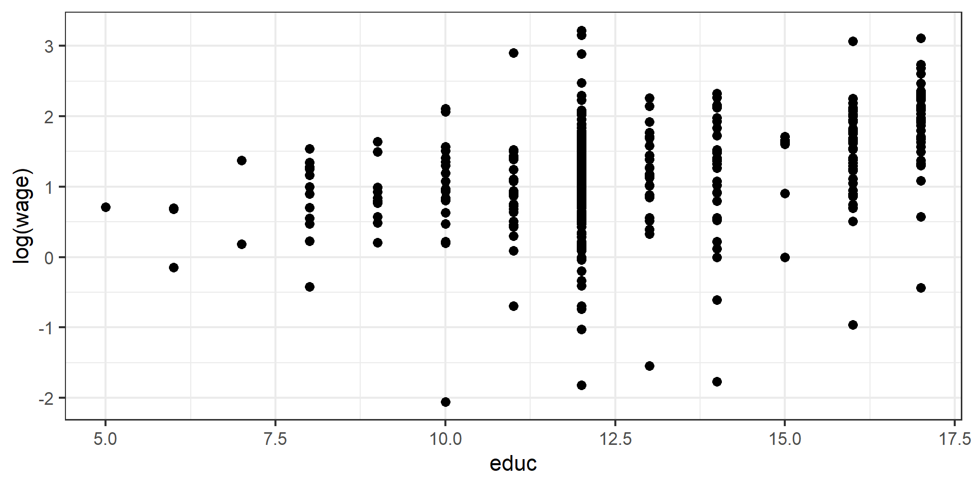
Case: Wage example

The origin model

Consider the following “error specified” wage model:

\[ \begin{align} lwage_i = \beta_1 +\beta_2educ_i + \beta_3exper_i +\beta_4expersq_i + e_i \end{align} \]

The difficulty with this model is that the error term may include some unobserved attributes, such as personal ability, that determine both wage and education.

In other words, the independent variable educ is correlated with the error term. And it is endogenous variable.

Note:

We will use years of schooling as the proxy variable of educ in practice, and it surely bring in error measurement issues as we have mentioned.

Consider the following error specified wage model, which the logarithmic (ˌlɒɡəˈrɪðmɪk) wage is the function of education,labor market experience and its quadratic term.As what we have discussed before. The difficulty with this model is that the error term may include some unobserved attributes, such as personal ability, that determine both wage and education.> There is one more thing we should remind. We will use years of schooling as the proxy variable of educ in practice, and it surely bring in error measurement issues as we have mentioned.Let us show all variables of our dataset.

Variables in dataset

With data set wooldridge::mroz, researchers were interest in the return to education for married women.

Other variables include father education, mother education, which are both measured by schooling years, etc (ɪt ˈsetərə).

Raw dataset

We will use 428 observations totally after delete rows with missing wage value.

Try yourself! Click and download the .csvfile

The scatter

The mis-specified model

The Assumed TRUE model is

\[ \begin{align} log(wage_i)=\beta_{0}+\beta_{1} edu_{i}+\beta_{2} exper_{i}+\beta_{3} exper^2_{i}+\beta_{4} ability_{i}+\epsilon_{i} \end{align} \]

Now, let’s consider the mis-specified model

\[ \begin{align} log(wage_i)=\alpha_{0}+\alpha_{1} edu_{i}+\alpha_{2} exper_{i}+\alpha_{3} exper^2_{i}+u_{i} \quad \text{(omitted ability)} \end{align} \]

• In the theory analysis, we have known that this model is mis-specified due to the important omitted variables(ability) and it will be dropped to the disturbance term\(u_i\).

• While the regressor edu is correlated with the disturbance term\(u_i\) (formally the omitted variables ability), thus the regressor edu is endogenous variable!

Using OLS method directly: tidy report

Of course, you can conduct the OLS regression directly without considering problems due to endogeneity, and may obtain the inconsistent estimators (as we have proved).

\[ \begin{aligned} \begin{split} lwage_i=&+\beta_{1}+\beta_{2}educ_i+\beta_{3}exper_i+\beta_{4}expersq_i+u_i \end{split} \end{aligned} \]

The OLS regression resuts is

\[ \begin{alignedat}{999} \begin{split} &\widehat{lwage}=&&-0.52&&+0.11educ_i&&+0.04exper_i&&-0.00expersq_i\\ &(s)&&(0.1986)&&(0.0141)&&(0.0132)&&(0.0004)\\ &(t)&&(-2.63)&&(+7.60)&&(+3.15)&&(-2.06)\\ &(over)&&n=428&&\hat{\sigma}=0.6664 && &&\\ &(fit)&&R^2=0.1568&&\bar{R}^2=0.1509 && &&\\ &(Ftest)&&F^*=26.29&&p=0.0000 && && \end{split} \end{alignedat} \]

This looks good, but we know it is not reliable due to endogeneity behind this “error specified” model.

You can type and run these R codes and then get the following tidy OLS results.You may see that:- The t statistic of estimators are given in this row.- And this row shows the standard error of the estimators.- The t test of all coefficients are significant with its abslute t value larger than 2.- And the F test is also significant with a small p value.This looks good, but we know it is not reliable due to endogeneity behind this “error specified” model.

Using OLS method directly: raw report

mod_origin <- formula(lwage ~ educ +exper+expersq)
ols_origin <- lm(formula = mod_origin, data = mroz)
summary(ols_origin)

17.3 IV and the choices

How to handle the endogenous variable problems?There is a way to go ahead, and we will resort to use instrumental variables in this section.

Instrumental Variable (IV)

problem and the motivation

We have seen that OLS estimator of\(\beta\) is inconsistent when one or more regressors is endogenous .

The problems of OLS arise because we imposed\(E(X_i\epsilon_i)=0\), which means we believe the sample data with

\[ \boldsymbol{X^{\prime} {e}=0} \]

When in fact error terms and regressors are correlated\(E(X_i\epsilon_i) \neq 0\).

conditions review

Suppose we can find a set of explanatory variables\(\boldsymbol{Z}\) satisfying two conditions:

• Relevance:\(\boldsymbol{Z}\) is correlated with\(\boldsymbol{X}\)

• Exogeneity:\(\boldsymbol{Z}\) is not correlated with\(\boldsymbol{\epsilon}\)

These variables (\(\boldsymbol{Z}\), in matrix form) can be used for consistent estimation and are known as Instrumental Variables (IV) .

IV Estimators

Our instrumental variable estimator,\(\hat{\beta}_{IV}\) is defined in terms of the following “normal equation” (moment condition, to be more precise)

\[ \begin{align} \boldsymbol{Z^{\prime} \hat{\epsilon}=Z^{\prime}\left(y-X \hat{\beta}_{IV}\right)=0} \end{align} \]

and thus, provided that\(Z^{\prime} X\) is square and non singular,

\[ \begin{align} \boldsymbol{\hat{\beta}_{IV}=\left(Z^{\prime} X\right)^{-1} Z^{\prime} y} \end{align} \]

The condition that\(\boldsymbol{Z^{\prime} X}\) is square and non singular, intuitively, is satisfied when we have as many instruments as regressors (a situation that is called exact identification).

However\(\boldsymbol{\hat{\beta}_{IV}}\) is generally biased in finite sample, but we can show that it is still consistent.

So let us prove this point.

Consistent estimator

\(\boldsymbol{\hat{\beta}_{IV}}\) is consistent. Since:

\[ \begin{align} \boldsymbol{\hat{\beta}_{IV} =\left(Z^{\prime} X\right)^{-1} Z^{\prime} y =\left(Z^{\prime} X\right)^{-1} Z^{\prime} (X\beta +\epsilon) =\beta+\left(Z^{\prime} X\right)^{-1} Z^{\prime} \epsilon} \end{align} \]

\[ \begin{align} p \lim \boldsymbol{{\hat{\beta}_{IV}}} &=\boldsymbol{\beta+p \lim \left(\left(Z^{\prime} X\right)^{-1} Z^{\prime} \epsilon\right)} \\ &=\boldsymbol{\beta+\left(p \lim \left(\frac{1}{n} Z^{\prime} X\right)\right)^{-1} \operatorname{plim}\left(\frac{1}{n} Z^{\prime} \epsilon\right) =\beta} \end{align} \]

• Relevance guarantees

\[ \begin{align} p \lim \left(\frac{1}{n} \boldsymbol{Z^{\prime} X}\right) &=p \lim \left(\frac{1}{n} \sum z_{i} X_{i}^{\prime}\right) \\ &=E\left(Z_{i} X_{i}^{\prime}\right) \neq 0 \end{align} \]

• Exogeneity ensures

\[ \begin{align} p \lim \left(\frac{1}{n} \boldsymbol{Z^{\prime} \epsilon}\right) &=p \lim \left(\frac{1}{n} \sum Z_{i} \epsilon_{i}\right) \\ &=E\left(Z_{i} \epsilon_{i}\right)=0 \end{align} \]

The IV estimator \(\boldsymbol{\hat{\beta}_{IV}}\) is consistent, Since the two instrument conditions are guaranteed .For simple, the instrument relevance condition guarantees correlation between \(Z_i\) and \(X_i\), and the instrument exogeneity condition ensures uncorrelations between \(Z_i\) and error term \(\epsilon_i\).Thus, the IV estimator is consistent under probability limits.

Inference

The natural estimator for\(\sigma^{2}\) is

\[ \begin{align} \hat{\sigma}_{I V}^{2} =\frac{\sum e_{i}^{2}}{n-k} =\frac{\boldsymbol{\left(y-X \hat{\beta}_{IV}\right)^{\prime}\left(y-X \hat{\beta}_{I V}\right)}}{n-k} \end{align} \]

can be shown to be consistent (not proved here).

Thus, we can perform hypothesis testing based on IV estimators\(\boldsymbol{\hat{\beta}_{IV}}\).

For the purpose of inference, we need to get the consistent estimate of the variance of disturbance \(\sigma^2\).The natural estimator for the variance of stochastic disturbance \(\sigma^{2}\) is \(\hat{\sigma}_{I V}^{2}\) as show below.And we don’t try to prove it here.After that, we can perform hypothesis testing based on IV estimators \(\boldsymbol{\hat{\beta}_{IV}}\).

Choices of instruments

However, finding valid instruments is the most difficult part of IV estimation in practice.

Good instruments need not only to be exogenous, but also need be highly correlative with the regressors.

Joke: If you can find a valid instrumental variable, you can get PhD from MIT.

Without a proof, we say that the asymptotic variance of\(\hat{\beta}_{I V}\) is

\[ \begin{align} \operatorname{Var}\left(\boldsymbol{\hat{\beta}_{I V}}\right)=\sigma^{2}\boldsymbol{\left(Z^{\prime} X\right)^{-1}\left(Z^{\prime} Z\right)\left(X^{\prime} Z\right)^{-1}} \end{align} \]

Where\(\boldsymbol{X^{\prime} Z}\) is the matrix of covariances between instruments and regressors.

If such correlation is low,\(\boldsymbol{X^{\prime} Z}\) will have elements close to zero and hence\(\boldsymbol{\left(X^{\prime} Z\right)^{-1}}\) will have huge elements. Thus,\(\operatorname{Var}\left(\boldsymbol{\hat{\beta}_{IV}}\right)\) will be very large.

So, what is the real challenge?___Without a proof, we say that the asymptotic (’æsɪmp,toʊtɪk) variance of \(\hat{\beta}_{I V}\) takes following output.If such correlation is low, this covariances matrix \(\boldsymbol{X^{\prime} Z}\) will have elements close to zero and hence its inverse matrix \(\boldsymbol{\left(X^{\prime} Z\right)^{-1}}\) will have huge elements.And then, the asymptotic variance of IV estimator \(\operatorname{Var}\left(\boldsymbol{\hat{\beta}_{IV}}\right)\) will be very large.This means the IV estimation will be useless.

Extension of choices

The common strategy is to construct\(\boldsymbol{Z}=(X_{ex}, X^{\ast})\) generally.

• Variables\(X_{ex}\) in\(\boldsymbol{X}=(X_{ex}, X_{en})\) are the assumed exogenous variables included in model.

• Other exogenous variables\(\boldsymbol{X^{\ast}}\) are “close” to the model, but do not enter the model explicitly.

If\(X\) can be shown to be exogenous, then\(X=Z\) and Gauss-Markov efficiency is recovered.

Instrumental Variable Estimators do not have any efficiency properties .

We can only talk about relative efficiency. It means that we can only choose the optimal set of instruments. Such that our estimator is the best we can obtain within all the class of possible instrumental variable estimators.

So, it is really big challenge to find the valid instruments and control the low level of asymptotic variance.While we can find a solution if we are luckly._We should remind one other thing._So we will ask that with what conditions we can excute this common strategy?

IV: Many available instruments

In case there are more instruments than endogenous variables (over-identification), we want to choose those instruments that have the highest correlation with\(X\) and hence give the lowest possible variance.

The best choice is obtained by using the fitted values of an OLS regression of each column of\(\boldsymbol{X}\) on all instruments\(\boldsymbol{Z}\), that is (after running\(k\) regressions, one for each column of\(\boldsymbol{X}\))

\[ \begin{align} \boldsymbol{\hat{X}=Z\left(Z^{\prime} Z\right)^{-1} Z^{\prime} X=ZF} \end{align} \]

We now use\(\boldsymbol{\hat{X}}\) as instrument, which is\(\boldsymbol{\hat{\beta}_{I V}=\left(\hat{X}^{\prime} X\right)^{-1} \hat{X}^{\prime} y}\)

We notice that (try to prove this):

\[ \begin{align} \boldsymbol{\hat{\beta}_{I V} =\left(\hat{X}^{\prime} X\right)^{-1} \hat{X}^{\prime} y=\left(X^{\prime} Z\left(Z^{\prime} Z\right)^{-1} Z^{\prime} X\right)^{-1} X^{\prime} Z\left(Z^{\prime} Z\right)^{-1} Z^{\prime} y } \end{align} \]

The clue is show below, and you may try to prove it.The last results show that when we have more instruments than endogenous variables \(\boldsymbol{\hat{\beta}_{IV}}\) can be computed in 2 steps (2SLS).

IV solution with omitted variables

Revall the wage case

Let’s go back to our example of the wage equation. Assume we are modeling wage as a function of education and ability.

\[ Wage_{i}=\beta_{0}+\beta_{1} Edu_{i}+\beta_{2} Abl_{i}+\epsilon_{i} \]

However, individual’s ability is clearly something that is not observed or measured and hence cannot be included in the model. since, ability is not included in the model it is included in the error term.

\[ Wage_{i}=\beta_{0}+\beta_{1} Edu_{i}+e_{i}, \quad \text {where} \quad e_{i}=\beta_{2} Abl_{i}+\epsilon_{i} \]

The problem is that ability not only affects wages but the more able individuals may spend more years in school, causing a positive correlation between the error term and education,\(\operatorname{cov}(Edu_i, e_i)>0\) .

Thus,\(Educ\) is an endogenous variable.

Conditions for valid instruments

If we can find a valid instrument for Educ we can estimate\(\beta_{1}\) using IV method. Suppose that we have a variable\(Z\) that satisfies the following conditions

• \(Z\) does not directly affect wages

• \(Z\) is uncorrelated with\(e\) (exogeneity), i.e.

\[ \operatorname{Cov}(e, z)=0 \quad \text{(4)} \]

since\(e_{i}=\beta_{2} Abl_{i}+\epsilon_{i}\),\(Z\) must be uncorrelated with ability.

-\(Z\) is (at least partially) correlated with the endogenous variable,i.e. Education (relevance),

\[ \operatorname{Cov}(Z, Edu) \neq 0 \quad \text{(5)} \]

Such condition can be tested(\(\alpha_2\)) by using a simple regression$:

\[ Edu_{i}=\alpha_{1}+\alpha_{2} Z_{i}+u_{i} \]

Then,\(Z\) is a valid instrument for\(Educ_i\). We showed earlier that the IV estimator of\(\beta_{1}\) is consistent.

And the instrumental variable \(Z\) should satisfies both relevance condition and exogeneity condition as we have mentioned before.So, what are these appropriate instruments for education?

Available options of instruments

Several economists have used family background variables as IVs for education.

• For example, mother’s education is positively correlated with child’s education, so it may satisfies condition of Relevance.

• Also, father’s education is positively correlated with child’s education, and it may satisfies condition of Relevance.

The problem is that mother’s or father ’s education might also be correlated with child’s ability(genetic inherited), in which case the condition of Exogeneity fails.

• Another IV for education that has been used by economists is the number of siblings while growing up.

Typically, having more siblings is associated with lower average levels of education and it should be uncorrelated with innate ability.

Anyway, it is worth to try using mother education as the instrument.

proxy variable model

Also, let us consider the case with measurement error in the independent variable.

For some reason, a variable\(X_i\) cannot be directly observed (data is not available), so it is common to find a imperfect measure(the proxy variable) for it.

The “real model” for wage is assumed to be:

\[ \begin {align} \log (Wage_i)=\beta_{0}+\beta_{1} Edu_i+\beta_{2} Abl_i+u_i \end {align} \]

However, since the ability variable (\(Abl_i\)) cannot be observed, we often replace it with the IQ level variable (\(IQ_i\)) and construct the following “proxy variable model” :

\[ \begin {align} \log (Wage_i)=\beta_{0}+\beta_{1} Edu_i+\beta_{2} IQ_i+u_i^{\ast} \end {align} \]

At this point, intelligence level\(IQ_i\) can be considered as a potential instrument for ability\(abil_i\).

NOT show because this case may cause confuse.Now we have got some available instruments, and the following question is how to process the IV estimation.In the next section, we will talk about Two-stage least squares method.

17.4 Two-stage least squares method

In this section, we will discuss how to perform Two-stage least squares estimation procedure.

Two-stage least squares

glance

When we have more instruments than endogenous variables,\(\boldsymbol{\hat{\beta}_{IV}}\) can be computed in 2 steps:

• Step 1: Regress each column of\(X\) on all the instruments (\(Z\) ,in matrix form ). For each column of\(X\), get the fitted values and combine them into the matrix\(\hat{X}\).

• Step 2: Regress\({Y}\) on\(\hat{X}\)

And, this procedure is named two-stage least squares or 2SLS or TSLS.

indentification

Consider the model setting

\[ \begin{align} Y_{i}=\beta_{0}+\sum_{j=1}^{k} \beta_{j} X_{j i}+\sum_{s=1}^{r} \beta_{k+s} W_{ri}+\epsilon_{i} \end{align} \]

where\(\left(X_{1 i}, \ldots, X_{k i}\right)\) are endogenous regressors,\(\left(W_{1 i}, \ldots, W_{r i}\right)\) are exogenous regressors and there are\(m\) instrumental variables\(\left(Z_{1 i}, \ldots, Z_{m i}\right)\) satisfying instrument relevance and instrument exogeneity conditions.

• When\(m=k\) ,the coefficients are exactly identified.

• When\(m>k\) ,the coefficients are overidentified.

• When\(m<k\), the coefficients are underidentified.

• Finnaly, coefficients can be identified only when\(m \geq k\).

Because the model identification is the most important thing before applying the estimation procedure.So, We should overview the model status explicitly.We will denote the general model format as below.

The procedure

• Stage 1: Regress\(X_{1i}\) on constant, all the instruments\(\left(Z_{1i}, \ldots, Z_{m i}\right)\) and all exogenous regressors\(\left(W_{1i}, \ldots, W_{ri}\right)\) using OLS and obtain the fitted values\(\hat{X}_{1 i}\) . Repeat this to get\(\left(\hat{X}_{1 i}, \ldots, \hat{X}_{k i}\right)\)

• Stage 2: Regress\(Y_{i}\) on constant,\(\left(\hat{X}_{1 i}, \ldots, \hat{X}_{k i}\right)\) and \(\left(W_{1 i}, \ldots, W_{r i}\right)\) usingOLS to obtain\(\left(\hat{\beta}_{0}^{IV}, \hat{\beta}_{1}^{IV}, \ldots, \hat{\beta}_{k+r}^{IV}\right)\)

So, in case with “exactly identification” and “over-identification”, we can go ahead with the Two-Stage Least Squares as a “whole” solution for IV estimation.

The solutions

We can conduct the 2SLS procedure with following two solutions:

• use the “Step-by-Step solution” methods without variance correction.

• use the “Integrated solution” with variance correction.

.notes[

Notice:

DO NOT use “Step-by-Step solution” solution in your paper! It is only for teaching purpose here.

In R ecosystem, we have two packages to execute the Integrated solution:

• We can use systemfit package function systemfit::systemfit().

• Or we may use ARE package function ARE::ivreg().

]

Let us apply these solutions to the empirical wage examples.

TSLS: Step-by-step solution

Stage 1: model

First, let’s try to use \(matheduc\) as instrument of endogenous variable \(educ\).

Stage 1 of 2SLS: with mother education as instrument

we can obtain the fitted variable \(\widehat{educ}\) by conduct the following step 1 OLS regression

\[ \begin{align} \widehat{educ} = \hat{\gamma}_1 +\hat{\gamma}_2exper + \hat{\gamma}_3expersq +\hat{\gamma}_4mothereduc \end{align} \]

Again, let us do the demo of two-stage least squares procedure based on the wage example.In the firs stage, we can obtain the fitted variable \(\widehat{educ}\) by conduct the following OLS regression.

Stage 1: OLS estimate

Here we obtain the OLS results of Stage 1 of 2SLS:

# modle setting
mod_step1 <- formula(educ~exper + expersq + motheduc)  
# OLS estimation
ols_step1 <- lm(formula = mod_step1, data = mroz)  

\[ \begin{alignedat}{999} \begin{split} &\widehat{educ}=&&+9.78&&+0.05exper_i&&-0.00expersq_i&&+0.27motheduc_i\\ &(s)&&(0.4239)&&(0.0417)&&(0.0012)&&(0.0311)\\ &(t)&&(+23.06)&&(+1.17)&&(-1.03)&&(+8.60)\\ &(fit)&&R^2=0.1527&&\bar{R}^2=0.1467 && &&\\ &(Ftest)&&F^*=25.47&&p=0.0000 && && \end{split} \end{alignedat} \]

The t -value for coefficient of \(mothereduc\) is so large (larger than 2), indicating a strong correlation between this instrument and the endogenous variable \(educ\) even after controlling for other variables.

we should note that the t-value for coefficient of \(mothereduc\) is larger than 2. and the t test is significant. This means there is a strong correlation between the instrument \(motheduc\) and the endogenous variable \(educ\) even when we control all other variables.

Stage 1: OLS predicted values

Along with the regression of Stage 1 of 2SLS, we will extract the fitted value \(\widehat{educ}\) and add them into new data set.

# add fitted educ to data set
mroz_add <- mroz %>% mutate(educHat = fitted(ols_step1)) 

Stage 2: model

Stage 2 of 2SLS: with mother education as instrument

In the second stage, we will regress log(wage) on the \(\widehat{educ}\) from stage 1 and experience and its quadratic term exp square.

\[ \begin{align} lwage = \hat{\beta}_1 +\hat{\beta}_2\widehat{educ} + \hat{\beta}_3exper +\hat{\beta}_4expersq + \hat{\epsilon} \end{align} \]

mod_step2 <- formula(lwage~educHat + exper + expersq)
ols_step2 <- lm(formula = mod_step2, data = mroz_add)

Stage 2: OLS estimate

By using the new data set (mroz_add), the result of the explicit 2SLS procedure are shown as below.

\[ \begin{alignedat}{999} \begin{split} &\widehat{lwage}=&&+0.20&&+0.05educHat_i&&+0.04exper_i&&-0.00expersq_i\\ &(s)&&(0.4933)&&(0.0391)&&(0.0142)&&(0.0004)\\ &(t)&&(+0.40)&&(+1.26)&&(+3.17)&&(-2.17)\\ &(fit)&&R^2=0.0456&&\bar{R}^2=0.0388 && &&\\ &(Ftest)&&F^*=6.75&&p=0.0002 && && \end{split} \end{alignedat} \]

Keep in mind, however, that the standard errors calculated in this way are incorrect (Why?).

while the t-test on the coefficient of education is not significant because the t statistics is less than the critical value 2. But the model F-test is significant with small p value here.

TSLS: Integrated solution

The whole story

We need a Integrated solution for following reasons:

• We should obtain the correct estimated error for test and inference.

• We should avoid tedious steps in the former step-by-step routine. When the model contains more than one endogenous regressors and there are lots available instruments, then the step-by-step solution will get extremely tedious.

The R toolbox

In R ecosystem, we have two packages to execute the integrated solution:

• We can use systemfit package function systemfit::systemfit().

• Or we may use ARE package function ARE::ivreg().

Both of these tools can conduct the integrated solution, and will adjust the variance of estimators automatically.

example 1: TSLS with only motheduc as IV

The TSLS model

In order to get the correct estimated error, we need use the “integrated solution” for 2SLS. And we will process the estimation with proper software and tools.

Firstly, let’s consider using \(motheduc\) as the only instrument for \(educ\).

\[ \begin{cases} \begin{align} \widehat{educ} &= \hat{\gamma}_1 +\hat{\gamma}_2exper + \hat{\gamma}_3expersq +\hat{\gamma}_4motheduc && \text{(stage 1)}\\ lwage & = \hat{\beta}_1 +\hat{\beta}_2\widehat{educ} + \hat{\beta}_3exper +\hat{\beta}_4expersq + \hat{\epsilon} && \text{(stage 2)} \end{align} \end{cases} \]

The TSLS results (tidy table)

• The t-test for variable educ is significant (p-value less than 0.05).

Note : The corresponding code of R programming is in the following slides. The table results use the report from the systemfit::systemfit() function.

The TSLS code: using R function systemfit::systemfit()

The R code using systemfit::systemfit() as follows:

# load pkg
require(systemfit)
# set two models
eq_1 <- educ ~  exper + expersq + motheduc
eq_2 <- lwage ~ educ + exper + expersq
sys <- list(eq1 = eq_1, eq2 = eq_2)
# specify the instruments
instr <- ~  exper + expersq + motheduc
# fit models
fit.sys <- systemfit(
sys, inst=instr,
method="2SLS", data = mroz)
# summary of model fit
smry.system_m <- summary(fit.sys)

The TSLS raw result: using R function systemfit::systemfit()

The following is the 2SLS analysis report using systemfit::systemfit():

smry.system_m

systemfit results 
method: 2SLS 

         N  DF     SSR detRCov   OLS-R2 McElroy-R2
system 856 848 2085.49 1.96552 0.150003   0.112323

      N  DF      SSR      MSE     RMSE       R2   Adj R2
eq1 428 424 1889.658 4.456742 2.111100 0.152694 0.146699
eq2 428 424  195.829 0.461861 0.679604 0.123130 0.116926

The covariance matrix of the residuals
         eq1      eq2
eq1 4.456742 0.304759
eq2 0.304759 0.461861

The correlations of the residuals
         eq1      eq2
eq1 1.000000 0.212418
eq2 0.212418 1.000000


2SLS estimates for 'eq1' (equation 1)
Model Formula: educ ~ exper + expersq + motheduc
Instruments: ~exper + expersq + motheduc

               Estimate  Std. Error  t value Pr(>|t|)    
(Intercept)  9.77510269  0.42388862 23.06055  < 2e-16 ***
exper        0.04886150  0.04166926  1.17260  0.24161    
expersq     -0.00128106  0.00124491 -1.02905  0.30404    
motheduc     0.26769081  0.03112980  8.59918  < 2e-16 ***
---
Signif. codes:  0 '***' 0.001 '**' 0.01 '*' 0.05 '.' 0.1 ' ' 1

Residual standard error: 2.1111 on 424 degrees of freedom
Number of observations: 428 Degrees of Freedom: 424 
SSR: 1889.658428 MSE: 4.456742 Root MSE: 2.1111 
Multiple R-Squared: 0.152694 Adjusted R-Squared: 0.146699 


2SLS estimates for 'eq2' (equation 2)
Model Formula: lwage ~ educ + exper + expersq
Instruments: ~exper + expersq + motheduc

                Estimate   Std. Error  t value  Pr(>|t|)   
(Intercept)  0.198186056  0.472877230  0.41911 0.6753503   
educ         0.049262953  0.037436026  1.31592 0.1889107   
exper        0.044855848  0.013576817  3.30386 0.0010346 **
expersq     -0.000922076  0.000406381 -2.26899 0.0237705 * 
---
Signif. codes:  0 '***' 0.001 '**' 0.01 '*' 0.05 '.' 0.1 ' ' 1

Residual standard error: 0.679604 on 424 degrees of freedom
Number of observations: 428 Degrees of Freedom: 424 
SSR: 195.829058 MSE: 0.461861 Root MSE: 0.679604 
Multiple R-Squared: 0.12313 Adjusted R-Squared: 0.116926 

NOTE : systemfit::systemfit() simultaneously reports the analysis results of two equations in 2SLS!

The TSLS code: using R function ARE::ivreg()

The R code using ARE::ivreg() as follows:

# load pkg
require(AER)
# specify model
mod_iv_m <- formula(lwage ~ educ + exper + expersq
| motheduc + exper + expersq)
# fit model
lm_iv_m <- ivreg(formula = mod_iv_m, data = mroz)
# summary of model fit
smry.ivm <- summary(lm_iv_m)

The TSLS code: using R function ARE::ivreg()

The following is the 2SLS analysis report using ARE::ivreg():

smry.ivm

Call:
ivreg(formula = mod_iv_m, data = mroz)

Residuals:
     Min       1Q   Median       3Q      Max 
-3.10804 -0.32633  0.06024  0.36772  2.34351 

Coefficients:
              Estimate Std. Error t value Pr(>|t|)   
(Intercept)  0.1981861  0.4728772   0.419  0.67535   
educ         0.0492630  0.0374360   1.316  0.18891   
exper        0.0448558  0.0135768   3.304  0.00103 **
expersq     -0.0009221  0.0004064  -2.269  0.02377 * 
---
Signif. codes:  0 '***' 0.001 '**' 0.01 '*' 0.05 '.' 0.1 ' ' 1

Residual standard error: 0.6796 on 424 degrees of freedom
Multiple R-Squared: 0.1231, Adjusted R-squared: 0.1169 
Wald test: 7.348 on 3 and 424 DF,  p-value: 8.228e-05 

We can see that the t-test for\(educ\) is not significant.We should note that the instruments (motheduc + exper + expersq) are included as whole behind the procedure in this code chunk. But we do not see these instruments in the output.We can see that the t-test on the coefficient of education is still not significant.

Note: ARE::ivreg() Only reports the result of the last equation of 2SLS, not include the first equation!

example 2: TSLS with only fatheduc as IV

The TSLS model

Now let’s consider using \(fatheduc\) as the only instrument for \(educ\).

\[ \begin{cases} \begin{align} \widehat{educ} &= \hat{\gamma}_1 +\hat{\gamma}_2exper + \hat{\gamma}_3expersq +\hat{\gamma}_4fatheduc && \text{(stage 1)}\\ lwage & = \hat{\beta}_1 +\hat{\beta}_2\widehat{educ} + \hat{\beta}_3exper +\hat{\beta}_4expersq + \hat{\epsilon} && \text{(stage 2)} \end{align} \end{cases} \]

We will repeat the whole procedure with R.

We will repeat the whole procedure with R.

The TSLS results (tidy table)

• The t-test for variable educ is significant (p-value less than 0.05).

Note : The corresponding code of R programming is in the following slides. The table results use the report from the systemfit::systemfit() function.

The TSLS code: using R function systemfit::systemfit()

The R code using systemfit::systemfit() as follows:

# load pkg
require(systemfit)
# set two models
eq_1 <- educ ~  exper + expersq + fatheduc
eq_2 <- lwage ~ educ + exper + expersq
sys <- list(eq1 = eq_1, eq2 = eq_2)
# specify the instruments
instr <- ~ exper + expersq + fatheduc
# fit models
fit.sys <- systemfit(
  formula = sys, inst=instr,
  method="2SLS", data = mroz
  )
# summary of model fit
smry.system_f <- summary(fit.sys)

The TSLS raw result: using R function systemfit::systemfit()

The following is the 2SLS analysis report using systemfit::systemfit():

smry.system_f

systemfit results 
method: 2SLS 

         N  DF     SSR detRCov   OLS-R2 McElroy-R2
system 856 848 2030.11 1.91943 0.172575   0.134508

      N  DF      SSR      MSE     RMSE       R2   Adj R2
eq1 428 424 1838.719 4.336602 2.082451 0.175535 0.169701
eq2 428 424  191.387 0.451384 0.671851 0.143022 0.136959

The covariance matrix of the residuals
         eq1      eq2
eq1 4.336602 0.195036
eq2 0.195036 0.451384

The correlations of the residuals
         eq1      eq2
eq1 1.000000 0.139402
eq2 0.139402 1.000000


2SLS estimates for 'eq1' (equation 1)
Model Formula: educ ~ exper + expersq + fatheduc
Instruments: ~exper + expersq + fatheduc

               Estimate  Std. Error  t value Pr(>|t|)    
(Intercept)  9.88703429  0.39560779 24.99201  < 2e-16 ***
exper        0.04682433  0.04110742  1.13907  0.25532    
expersq     -0.00115038  0.00122857 -0.93636  0.34962    
fatheduc     0.27050610  0.02887859  9.36701  < 2e-16 ***
---
Signif. codes:  0 '***' 0.001 '**' 0.01 '*' 0.05 '.' 0.1 ' ' 1

Residual standard error: 2.082451 on 424 degrees of freedom
Number of observations: 428 Degrees of Freedom: 424 
SSR: 1838.719104 MSE: 4.336602 Root MSE: 2.082451 
Multiple R-Squared: 0.175535 Adjusted R-Squared: 0.169701 


2SLS estimates for 'eq2' (equation 2)
Model Formula: lwage ~ educ + exper + expersq
Instruments: ~exper + expersq + fatheduc

                Estimate   Std. Error  t value  Pr(>|t|)   
(Intercept) -0.061116933  0.436446128 -0.14003 0.8887003   
educ         0.070226291  0.034442694  2.03893 0.0420766 * 
exper        0.043671588  0.013400121  3.25904 0.0012079 **
expersq     -0.000882155  0.000400917 -2.20034 0.0283212 * 
---
Signif. codes:  0 '***' 0.001 '**' 0.01 '*' 0.05 '.' 0.1 ' ' 1

Residual standard error: 0.671851 on 424 degrees of freedom
Number of observations: 428 Degrees of Freedom: 424 
SSR: 191.386653 MSE: 0.451384 Root MSE: 0.671851 
Multiple R-Squared: 0.143022 Adjusted R-Squared: 0.136959 

NOTE : systemfit::systemfit() simultaneously reports the analysis results of two equations in 2SLS!

The TSLS code: using R function ARE::ivreg()

The R code using ARE::ivreg() as follows:

# load pkg
require(AER)
# specify model
mod_iv_f <- formula(
  lwage ~ educ + exper + expersq
  | fatheduc + exper + expersq
  )
# fit model
lm_iv_f <- ivreg(formula = mod_iv_f, data = mroz)
# summary of model fit
smry.ivf <- summary(lm_iv_f)

We can see the insturments (fatheduc + exper + expersq) are included as whole behind the procedure in this code chunk.While, We can find that the t-test on the coefficient of education is significant now with its p value less than 0.05.

The TSLS raw result: using R function ARE::ivreg()

The following is the 2SLS analysis report using ARE::ivreg():

smry.ivf

Call:
ivreg(formula = mod_iv_f, data = mroz)

Residuals:
     Min       1Q   Median       3Q      Max 
-3.09170 -0.32776  0.05006  0.37365  2.35346 

Coefficients:
              Estimate Std. Error t value Pr(>|t|)   
(Intercept) -0.0611169  0.4364461  -0.140  0.88870   
educ         0.0702263  0.0344427   2.039  0.04208 * 
exper        0.0436716  0.0134001   3.259  0.00121 **
expersq     -0.0008822  0.0004009  -2.200  0.02832 * 
---
Signif. codes:  0 '***' 0.001 '**' 0.01 '*' 0.05 '.' 0.1 ' ' 1

Residual standard error: 0.6719 on 424 degrees of freedom
Multiple R-Squared: 0.143,  Adjusted R-squared: 0.137 
Wald test: 8.314 on 3 and 424 DF,  p-value: 2.201e-05 

Note: ARE::ivreg() Only reports the result of the last equation of 2SLS, not include the first equation!

example 3: TSLS with both mothedu and fatheduc as IVs

The TSLS model

Also, we can use both \(motheduc\) and \(fatheduc\) as instruments for \(educ\).

\[ \begin{cases} \begin{align} \widehat{educ} &= \hat{\gamma}_1 +\hat{\gamma}_2exper + \hat{\beta}_3expersq +\hat{\beta}_4motheduc + \hat{\beta}_5fatheduc && \text{(stage 1)}\\ lwage & = \hat{\beta}_1 +\hat{\beta}_2\widehat{educ} + \hat{\beta}_3exper +\hat{\beta}_4expersq + \hat{\epsilon} && \text{(stage 2)} \end{align} \end{cases} \]

The TSLS results (tidy table)

We can see that the t-test result of the coefficient of variable educ is significant (p-value less than 0.1).The insturments (motheduc +fatheduc + exper + expersq) are included behind the procedure in this code chunk.And we can find that the t-test on the coefficient of education is significant with its p value less than 0.1.

Note : The corresponding code of R programming is in the following slides. The table results use the report from the systemfit::systemfit() function.

The TSLS code: using R function systemfit::systemfit()

The R code using systemfit::systemfit() as follows:

# load pkg
require(systemfit)
# set two models
eq_1 <- educ ~ exper + expersq + motheduc + fatheduc
eq_2 <- lwage ~ educ + exper + expersq
sys <- list(eq1 = eq_1, eq2 = eq_2)
# specify the instruments
instr <- ~ exper + expersq + motheduc + fatheduc
# fit models
fit.sys <- systemfit(
sys, inst=instr,
method="2SLS", data = mroz)
# summary of model fit
smry.system_mf <- summary(fit.sys)

The TSLS raw result: using R function systemfit::systemfit()

The following is the 2SLS analysis report using systemfit::systemfit():

smry.system_mf

systemfit results 
method: 2SLS 

         N  DF    SSR detRCov   OLS-R2 McElroy-R2
system 856 847 1951.6 1.83425 0.204575   0.149485

      N  DF     SSR      MSE     RMSE       R2   Adj R2
eq1 428 423 1758.58 4.157388 2.038967 0.211471 0.204014
eq2 428 424  193.02 0.455236 0.674712 0.135708 0.129593

The covariance matrix of the residuals
         eq1      eq2
eq1 4.157388 0.241536
eq2 0.241536 0.455236

The correlations of the residuals
         eq1      eq2
eq1 1.000000 0.175571
eq2 0.175571 1.000000


2SLS estimates for 'eq1' (equation 1)
Model Formula: educ ~ exper + expersq + motheduc + fatheduc
Instruments: ~exper + expersq + motheduc + fatheduc

               Estimate  Std. Error  t value   Pr(>|t|)    
(Intercept)  9.10264011  0.42656137 21.33958 < 2.22e-16 ***
exper        0.04522542  0.04025071  1.12359    0.26182    
expersq     -0.00100909  0.00120334 -0.83857    0.40218    
motheduc     0.15759703  0.03589412  4.39061 1.4298e-05 ***
fatheduc     0.18954841  0.03375647  5.61517 3.5615e-08 ***
---
Signif. codes:  0 '***' 0.001 '**' 0.01 '*' 0.05 '.' 0.1 ' ' 1

Residual standard error: 2.038967 on 423 degrees of freedom
Number of observations: 428 Degrees of Freedom: 423 
SSR: 1758.575263 MSE: 4.157388 Root MSE: 2.038967 
Multiple R-Squared: 0.211471 Adjusted R-Squared: 0.204014 


2SLS estimates for 'eq2' (equation 2)
Model Formula: lwage ~ educ + exper + expersq
Instruments: ~exper + expersq + motheduc + fatheduc

                Estimate   Std. Error  t value  Pr(>|t|)   
(Intercept)  0.048100307  0.400328078  0.12015 0.9044195   
educ         0.061396629  0.031436696  1.95302 0.0514742 . 
exper        0.044170393  0.013432476  3.28833 0.0010918 **
expersq     -0.000898970  0.000401686 -2.23799 0.0257400 * 
---
Signif. codes:  0 '***' 0.001 '**' 0.01 '*' 0.05 '.' 0.1 ' ' 1

Residual standard error: 0.674712 on 424 degrees of freedom
Number of observations: 428 Degrees of Freedom: 424 
SSR: 193.020015 MSE: 0.455236 Root MSE: 0.674712 
Multiple R-Squared: 0.135708 Adjusted R-Squared: 0.129593 

NOTE : systemfit::systemfit() simultaneously reports the analysis results of two equations in 2SLS!

The TSLS code: using R function ARE::ivreg()

The R code using ARE::ivreg() as follows:

The TSLS raw result: using R functionARE::ivreg()

The following is the 2SLS analysis report using ARE::ivreg():

smry.ivmf

Call:
ivreg(formula = mod_iv_mf, data = mroz)

Residuals:
    Min      1Q  Median      3Q     Max 
-3.0986 -0.3196  0.0551  0.3689  2.3493 

Coefficients:
              Estimate Std. Error t value Pr(>|t|)   
(Intercept)  0.0481003  0.4003281   0.120  0.90442   
educ         0.0613966  0.0314367   1.953  0.05147 . 
exper        0.0441704  0.0134325   3.288  0.00109 **
expersq     -0.0008990  0.0004017  -2.238  0.02574 * 
---
Signif. codes:  0 '***' 0.001 '**' 0.01 '*' 0.05 '.' 0.1 ' ' 1

Residual standard error: 0.6747 on 424 degrees of freedom
Multiple R-Squared: 0.1357, Adjusted R-squared: 0.1296 
Wald test: 8.141 on 3 and 424 DF,  p-value: 2.787e-05 

Note: ARE::ivreg() Only reports the result of the last equation of 2SLS, not include the first equation!

Solutions comparison

Glance of mutiple models

Until now, we obtain totally Five estimation results with different model settings or solutions:

1. Error specification model with OLS regression directly.

2. (Step-by-Step solution) Explicit 2SLS estimation without variance correction (IV regression step by step with only \(matheduc\) as instrument).

3. (Integrated solution) Dedicated IV estimation with variance correction ( using R tools of systemfit::systemfit() or ARE::ivreg()).

• The IV model with only\(motheduc\) as instrument for endogenous variable \(edu\)

• The IV model with only\(fatheduc\) as instrument for endogenous variable \(edu\)

• The IV model with both\(motheduc\) and\(fatheduc\) as instruments

For the purpose of comparison, all results will show in next slide.

we use R function ARE::ivreg() to get the IV estimation with variance correction with the last three model considering different instruments.

tidy reports (png)

Stidy reports (html)

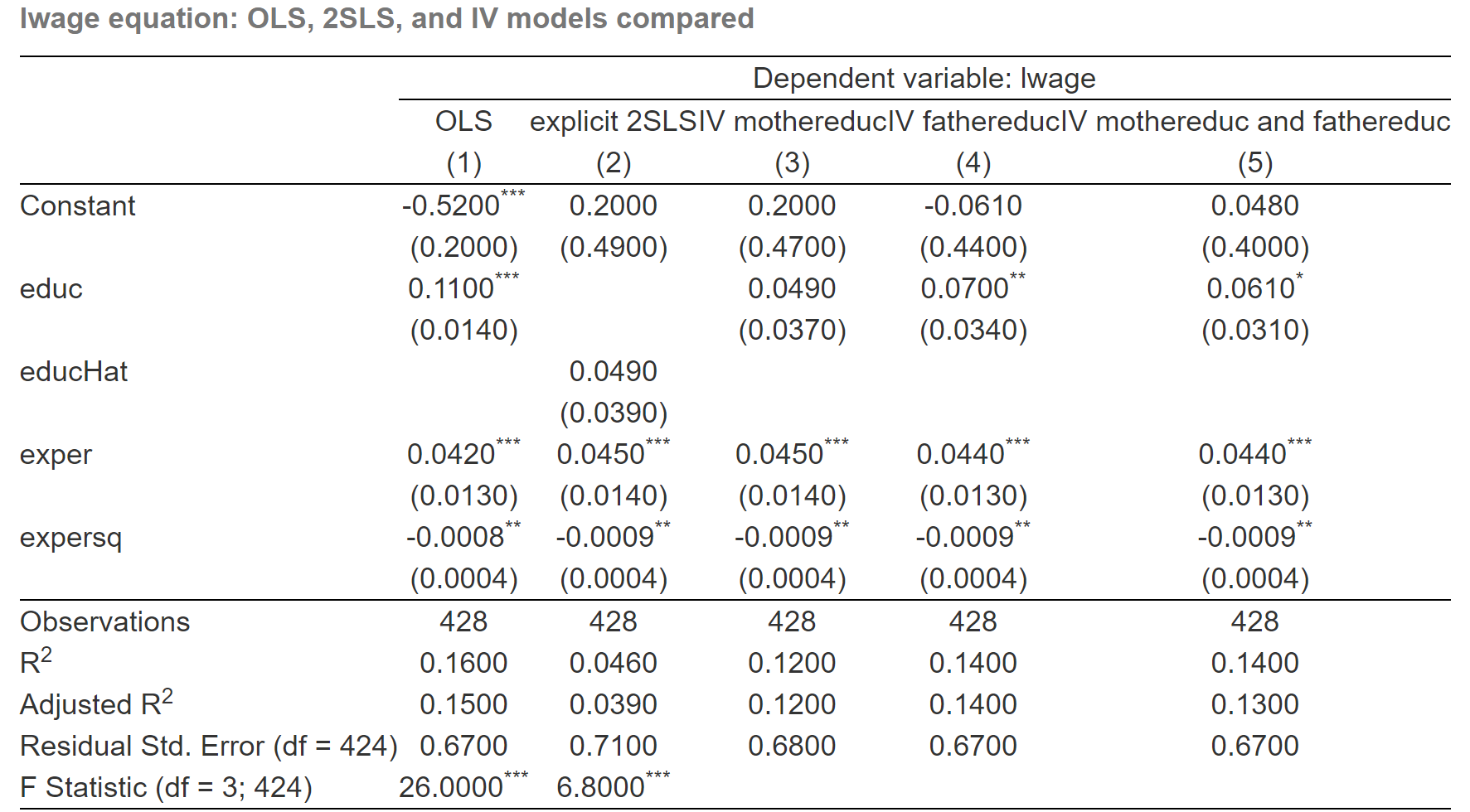
	Dependent variable: lwage
	OLS	explicit 2SLS	IV mothereduc	IV fathereduc	IV mothereduc and fathereduc
	(1)	(2)	(3)	(4)	(5)
Constant	-0.5220***	0.1982	0.1982	-0.0611	0.0481
	(0.1986)	(0.4933)	(0.4729)	(0.4364)	(0.4003)
educ	0.1075***		0.0493	0.0702**	0.0614*
	(0.0141)		(0.0374)	(0.0344)	(0.0314)
educHat		0.0493
		(0.0391)
exper	0.0416***	0.0449***	0.0449***	0.0437***	0.0442***
	(0.0132)	(0.0142)	(0.0136)	(0.0134)	(0.0134)
expersq	-0.0008**	-0.0009**	-0.0009**	-0.0009**	-0.0009**
	(0.0004)	(0.0004)	(0.0004)	(0.0004)	(0.0004)
Observations	428	428	428	428	428
R2	0.1568	0.0456	0.1231	0.1430	0.1357
Adjusted R2	0.1509	0.0388	0.1169	0.1370	0.1296
Residual Std. Error (df = 424)	0.6664	0.7090	0.6796	0.6719	0.6747
F Statistic (df = 3; 424)	26.2862***	6.7510***

see online book “Principles of Econometrics with R”（10.1 The Instrumental Variables (IV) Method，free online）

Report tips

• The second column shows the result of the direct OLS estimation, and the third column shows the result of explicit 2SLS estimation without variance correction.

• While the last three column shows the results of IV solution with variance correction.

• And we should also remind that the \(educ\) in the IV model is equivalent to the \(educHat\) in 2SLS.

• The value within the bracket is the standard error of the estimator.

Report insights

So the key points of this comparison including:

• Firstly, the table shows that the importance of education in determining wage decreases in the IV model (3) (4) and (5) with the coefficients 0.049, 0.07, 0.061 respectively. And the standard error also decrease along IV estimation (3) , (4) and (5).

• Secondly, It also shows that the explicit 2SLS model (2) and the IV model with only \(motheduc\) instrument yield the same coefficients, but the standard errors are different. The standard error in explicit 2SLS is 0.039, which is little large than the standard error 0.037 in IV estimation.

• Thirdly, the t-test of the coefficient on education shows no significance when we use motheduc as the only instrument for education. You can compare this under the explicit 2SLS estimation or IV estimation.

• Fourthly, we can fully feel and understand the relative estimated efficiency of 2SLS!

Further thinking

After the empirical comparison, we will be even more confused with these results.

While, new question will arise inside our mind.

• Which estimation is the best?

• How to judge and evaluate different instrument choices?

We will discuss these topics in the next section.

17.5 Testing Instrument validity

As we know, valid instruments should satisfy both relevance condition and exogeneity condition.So, let us check these conditions in this section.

Instrument vality

Consider the general model

\[ \begin{align} Y_{i}=\beta_{0}+\sum_{j=1}^{k} \beta_{j} X_{j i}+\sum_{s=1}^{r} \beta_{k+s} W_{ri}+\epsilon_{i} \end{align} \]

• \(Y_{i}\) is the dependent variable
• \(\beta_{0}, \ldots, \beta_{k+1}\) are \(1+k+r\) unknown regression coefficients
• \(X_{1 i}, \ldots, X_{k i}\) are \(k\) endogenous regressors
• \(W_{1 i}, \ldots, W_{r i}\) are \(r\) exogenous regressors which are uncorrelated with \(u_{i}\)
• \(u_{i}\) is the error term
• \(Z_{1 i}, \ldots, Z_{m i}\) are \(m\) instrumental variables

Instrument valid means satisfy both Relevance and Exogeneity conditions.

\[ E\left(Z_{i} X_{i}^{\prime}\right) \neq 0 \]

\[ E\left(Z_{i} \epsilon_{i}\right)=0 \]

Consider the general model as we have done.

Instrument Relevance

In practice, Instrument Relevance also means that:

If there are\(k\) endogenous variables and\(m\) instruments\(Z\), and\(m \geq k\), it must hold that the exogenous vector

\[ \left(\hat{X}_{1 i}^{*}, \ldots, \hat{X}_{k i}^{*}, W_{1 i}, \ldots, W_{r i}, 1\right) \]

should not be perfectly multicollinear.

Where: - \(\hat{X}_{1i}^{\ast}, \ldots, \hat{X}_{ki}^{\ast}\) are the predicted values from the \(k\) first stage regressions. - 1 denotes the constant regressor which equals 1 for all observations.

While the concept of Instrument Relevance is much tricky.So, what is the meaning of Instrument Relevance?___Obviously, the perfect multicollinear is the rare fact and can be get rid with careful inspection.What we really need to pay attention is the contrary fact which is called weak instruments.

Weak instrument: introduction

Definition

Instruments that explain little variation in the endogenous regressor \(X\) are called weak instruments.

Formally, When\(\operatorname{corr}\left(Z_{i}, X_{i}\right)\) is close to zero,\(z_{i}\) is called a weak instrument.

• Consider a simple one regressor model\(Y_{i}=\beta_{0}+\beta_{1} X_{i}+\epsilon_{i}\)

• The IV estimator of\(\beta_{1}\) is\(\widehat{\beta}_{1}^{IV}=\frac{\sum_{i=1}^{n}\left(Z_{i}-\bar{Z}\right)\left(Y_{i}-\bar{Y}\right)}{\sum_{i=1}^{n}\left(Z_{i}-\bar{Z}\right)\left(X_{i}-\bar{X}\right)}\)

Note that\(\frac{1}{n} \sum_{i=1}^{n}\left(Z_{i}-\bar{Z}\right)\left(Y_{i}-\bar{Y}\right) \xrightarrow{p} \operatorname{Cov}\left(Z_{i}, Y_{i}\right)\)

and\(\frac{1}{n} \sum_{i=1}^{n}\left(Z_{i}-\bar{Z}\right)\left(X_{i}-\bar{X}\right) \xrightarrow{p} \operatorname{Cov}\left(Z_{i}, X_{i}\right)\).

• Thus,if\(\operatorname{Cov}\left(Z_{i},X_{i}\right) \approx 0\), then \(\widehat{\beta}_{1}^{IV}\) is useless.

Let me give you an example.

Weak instrument: Birth weight example

Edogeneity and choice of instrument

We focus on the effect of cigarette smoking on the infant birth weight. Without other explanatory variables, the model is

-\(bwght =\) child birth weight, in ounces.

-\(packs =\) packs smoked per day while pregnant.

-\(cigprice=\) cigarette price in home state

\[ \begin{align} \log (\text {bwght})=\beta_{0}+\beta_{1} \text {packs}+u_{i} \end{align} \]

• We might worry that packs is cor-related with other health factors or the availability of good prenatal care, so that\(packs\) and\(u_i\) might be correlated.

• A possible instrumental variable for\(packs\) is the average price of cigarettes (\(cigprice\)) in the state . We will assume that\(cigprice\) and\(u_i\) are uncorrelated.

the assumed TRUE model may be\[ \begin{align}\log (\text {bwght})=\beta_{0}+\beta_{1} \text {packs}+ ( \beta_2 care\_surport)+u_{i}\end{align} \]-\(cigs =\) number of cigarettes smoked by the mother while pregnant, per day.-\(faminc=\) annual family income, in thousands of dollars.

We will use data set from wooldridge::bwght.

TSLS estimation

However, by regressing \(packs\) on \(cigprice\) in stage 1, we find basically no effect.

\[ \begin{alignedat}{999} \begin{split} &\widehat{packs}=&&+0.0674&&+0.0003cigprice_i\\ &(s)&&(0.1025)&&(0.0008)\\ &(t)&&(+0.66)&&(+0.36)\\ &(Ftest)&&F^*=0.13&&p=0.7179 \end{split} \end{alignedat} \]

If we insist to use \(cigprice\) as instrument, and run the stage 2 OLS, we will find

\[ \begin{alignedat}{999} \begin{split} &\widehat{lbwght}=&&+4.4481&&+2.9887packs\_hat_i\\ &(s)&&(0.1843)&&(1.7654)\\ &(t)&&(+24.13)&&(+1.69)\\ &(Ftest)&&F^*=2.87&&p=0.0907 \end{split} \end{alignedat} \]

• because there is huge standard error and not significant on coefficient of packs.- and also it has the wrong sign on coefficient of packs, which should not be positive.As what we have discussed, the result is unbelievable since the cigprice is a weak instrument for packs.

Obviously, this estimation is meaningless (Why?).The \(cigprice\) behaves as a weak instrument, and the problem was already exposed in stage 1 regression.

The strategy with weak instruments

The weak instrument (\(Z_i\) and\(X_i\) is week correlated) led to an important finding: even with very large sample sizes the 2SLS estimator can be biased and a distribution that is very different from standard normal (Staiger and Stock 1997).

There are two ways to proceed if instruments are weak:

• Discard the weak instruments and/or find stronger instruments.

While the former is only an option if the unknown coefficients remain identified when the weak instruments are discarded, the latter can be difficult and even may require a redesign of the whole study.

• Stick with the weak instruments but use methods that improve upon TSLS.

Such as limited information maximum likelihood estimation (LIML).

So, what should we do if the instruments are weak or some of them are weak?

Weak instrument test (solution 1): Restricted F-test

Test situation: Only one endogenous regressor in the model

In case with a single endogenous regressor, we can take the F-test to check the Weak instrument.

The basic idea of the F-test is very simple:

If the estimated coefficients of all instruments in the first-stage of a 2SLS estimation are zero, the instruments do not explain any of the variation in the\(X\) which clearly violates the relevance assumption.

Test procudure

We may use the following rule of thumb:

• Conduct the first-stage regression of a 2SLS estimation

\[ \begin{align} X_{i}=\hat{\gamma}_{0}+\hat{\gamma}_{1} W_{1 i}+\ldots+\hat{\gamma}_{p} W_{p i}+ \hat{\theta}_{1} Z_{1 i}+\ldots+\hat{\theta}_{q} Z_{q i}+v_{i} \quad \text{(3)} \end{align} \]

• Test the restricted joint hypothesis\(H_0: \hat{\theta}_1=\ldots=\hat{\theta}_q=0\) by compute the\(F\)-statistic. We call this Restricted F-test which is different with the Classical overall F-test.

• If the\(F\)-statistic is less than critical value, the instruments are weak.

The rule of thumb is easily implemented in R. Run the first-stage regression using lm() and subsequently compute the restricted \(F\)-statistic by R function of car::linearHypothesis().

Also, you may ask that how do you know the instruments are weak or some of them are weak?We will test this considering with different situations.

The Classical overall F-test has\(H_0:\gamma_1 = \cdots = \gamma_p =\hat{\theta}_1=\ldots=\hat{\theta}_q=0\)

Weak instrument test (solution 1): Restricted F-test on wage example

Model setting

For all three IV model, we can test instrument(s) relevance respectively.

\[ \begin{align} educ &= \gamma_1 +\gamma_2exper +\gamma_2expersq + \theta_1motheduc +v && \text{(relevance test 1)}\\ educ &= \gamma_1 +\gamma_2exper +\gamma_2expersq + \theta_2fatheduc +v && \text{(relevance test 2)} \\ educ &= \gamma_1 +\gamma_2exper +\gamma_2expersq + \theta_1motheduc + \theta_2fatheduc +v && \text{(relevance test 3)} \end{align} \]

And we will test the weak instrument issues by using restricted F test.

motheduc IV: Restricted F-test(model and hypothesis)

Consider model 1:

\[ \begin{align} educ &= \gamma_1 +\gamma_2exper +\gamma_3expersq + \theta_1motheduc +v \end{align} \]

The restricted F-test’ null hypothesis:\(H_0: \theta_1 =0\).

We will test whether motheduc are week instruments.

motheduc IV: Restricted F-test(R Code and result)

The result show that the p-value of\(F^{\ast}\) is much smaller than 0.01. Null hypothesis \(H_0\) was rejected. motheduc is instruments relevance (exogeneity valid).

library("car")
mod_relevance1 <- formula(educ ~ exper +expersq + motheduc)
ols_relevance1 <- lm(formula = mod_relevance1, data = mroz)
ftest_constrain_m <- linearHypothesis(
  ols_relevance1, 
  c("motheduc=0")
  )

Linear hypothesis test:
motheduc = 0

Model 1: restricted model
Model 2: educ ~ exper + expersq + motheduc

  Res.Df    RSS Df Sum of Sq      F    Pr(>F)    
1    425 2219.2                                  
2    424 1889.7  1    329.56 73.946 < 2.2e-16 ***
---
Signif. codes:  0 '***' 0.001 '**' 0.01 '*' 0.05 '.' 0.1 ' ' 1

Test comparision: Classic F-test (hypothsis and result)

\[ \begin{align} educ &= \gamma_1 +\gamma_2exper +\gamma_2expersq + \theta_1motheduc +v \end{align} \]

The classic OLS F-test’ null hypothesis:\(H_0: \gamma_2 = \gamma_3= \theta_1 =0\).

The OLS estimation results are:

\[ \begin{alignedat}{999} \begin{split} &\widehat{educ}=&&+9.78&&+0.05exper_i&&-0.00expersq_i&&+0.27motheduc_i\\ &(s)&&(0.4239)&&(0.0417)&&(0.0012)&&(0.0311)\\ &(t)&&(+23.06)&&(+1.17)&&(-1.03)&&(+8.60) \end{split} \end{alignedat} \]

Restricted F test take the Null hypotheis with coefficients before the instruments all euqal to zero, While the classical F test take the Null hypotheis with coefficients before all regressors equal to zero.

fatheduc IV: Restricted F-test (model and hypothesis)

Consider model 2:

\[ \begin{align} educ &= \gamma_1 +\gamma_2exper +\gamma_3expersq + \theta_1fatheduc +v && \text{(relevance test 2)} \end{align} \]

The restricted F-test’ null hypothesis:\(H_0: \theta_1 =0\).

We will test whether fatheduc are week instruments.

fatheduc IV: Restricted F-test (R Code and result)

The result show that the p-value of\(F^{\ast}\) is much smaller than 0.01. Null hypothesis \(H_0\) was rejected. fatheduc is instruments relevance (exogeneity valid).

mod_relevance2 <- formula(educ ~ exper +expersq  + fatheduc)
ols_relevance2 <- lm(formula = mod_relevance2, data = mroz)
ftest_constrain_f <- linearHypothesis(
  ols_relevance2, c("fatheduc=0")
  )

Linear hypothesis test:
fatheduc = 0

Model 1: restricted model
Model 2: educ ~ exper + expersq + fatheduc

  Res.Df    RSS Df Sum of Sq      F    Pr(>F)    
1    425 2219.2                                  
2    424 1838.7  1     380.5 87.741 < 2.2e-16 ***
---
Signif. codes:  0 '***' 0.001 '**' 0.01 '*' 0.05 '.' 0.1 ' ' 1

motheduc and fatheduc IV: restricted F-test (model and hypothesis)

Consider model 3:

\[ \begin{align} educ &= \gamma_1 +\gamma_2exper +\gamma_3expersq + \theta_1motheduc + \theta_2fatheduc +v && \text{(relevance test 3)} \end{align} \]

The restricted F-test’ null hypothesis:\(H_0: \theta_1 = \theta_2 =0\).

We will test whether motheduc and fatheduc are week instruments.

motheduc and fatheduc IV: restricted F-test (R code and result)

The result show that the p-value of\(F^{\ast}\) is much smaller than 0.01. Null hypothesis \(H_0\) was rejected. fatheduc and motheduc are instruments relevance (exogeneity valid).

mod_relevance3 <- formula(educ ~ exper +expersq + motheduc + fatheduc)
ols_relevance3 <- lm(formula = mod_relevance3, data = mroz)
ftest_constrain_mf <- linearHypothesis(
  ols_relevance3, 
  c("motheduc=0", "fatheduc=0")
)

Linear hypothesis test:
motheduc = 0
fatheduc = 0

Model 1: restricted model
Model 2: educ ~ exper + expersq + motheduc + fatheduc

  Res.Df    RSS Df Sum of Sq    F    Pr(>F)    
1    425 2219.2                                
2    423 1758.6  2    460.64 55.4 < 2.2e-16 ***
---
Signif. codes:  0 '***' 0.001 '**' 0.01 '*' 0.05 '.' 0.1 ' ' 1

In sum, all relecance model test are significant. And we can conclude that the instrumenta mothereducation and father education satisify the relevance condition.Until now, we show the relevance F-test with situation that contains only one endogenous regressor.Next, I will give a two endogeous variables example by using Cragg-Donald test.

Weak instrument test (solution 2): Cragg-Donald test

Test situation: More than one endogenous regressor in the model

The former test for weak instruments might be unreliable with more than one endogenous regressor, though, because there is indeed one\(F\)-statistic for each endogenous regressor.

Test procedure

An alternative is the Cragg-Donald test based on the following statistic:

\[ \begin{align} F=\frac{N-G-B}{L} \frac{r_{B}^{2}}{1-r_{B}^{2}} \end{align} \]

• where:\(G\) is the number of exogenous regressors;\(B\) is the number of endogenous regressors;\(L\) is the number of external instruments;\(r_B\) is the lowest canonical correlation.

Canonical correlation is a measure of the correlation between the endogenous and the exogenous variables, which can be calculated by the function cancor() in R.

external (ɪkˈstɜːnl)Canonical (kəˈnɒnɪkl)

Weak instrument test (solution 2): Crag-Donald test on Work hour example

Case backgound

Let us construct another IV model with two endogenous regressors. We assumed the following work hours determination model:

\[ \begin{equation} hushrs=\beta_{1}+\beta_{2} mtr+\beta_{3} educ+\beta_{4} kidsl6+\beta_{5} nwifeinc+e \end{equation} \]

• \(hushrs\): work hours of husband, 1975
• \(mtr\): federal marriage tax rate on woman
• \(kidslt6\): have kids < 6 years (dummy variable)
• \(nwifeinc\): wife’s net income

There are:

• Two endogenous variables: \(educ\) and \(mtr\)
• Two exogenous regressors: \(nwifeinc\) and \(kidslt6\)
• And two external instruments: \(motheduc\) and \(fatheduc\).

Cragg-Donald test: R code

The data set is still mroz, restricted to women that are in the labor force(\(inlf=1\)).

# filter samples
mroz1 <- wooldridge::mroz %>% 
  filter(wage>0, inlf==1)
# set parameters
N <- nrow(mroz1); G <- 2; B <- 2; L <- 2
# for endogenous variables
x1 <- resid(lm( mtr ~ kidslt6 + nwifeinc, data = mroz1))
x2 <- resid(lm( educ ~ kidslt6 + nwifeinc, data = mroz1))
# for instruments
z1 <-resid(lm(motheduc ~ kidslt6 + nwifeinc, data = mroz1))
z2 <-resid(lm(fatheduc ~ kidslt6 + nwifeinc, data=mroz1))
# column bind
X <- cbind(x1,x2)
Y <- cbind(z1,z2)
# calculate Canonical correlation
rB <- min(cancor(X,Y)$cor)
# obtain the F statistics
CraggDonaldF <- ((N-G-L)/L)/((1-rB^2)/rB^2)

Cragg-Donald test: R result

Run these code lines, we can obtain the results:

Table 1: Cragg-Donald test results

G	L	B	N	rb	CraggDonaldF
2	2	2	428	0.0218	0.1008

The result show the Cragg-Donald \(F=\) 0.1008 , which is much smaller than the critical value 4.58^[1].

This test can not rejects the null hypothesis, thus we may conclude that some of these instruments are weak.

You can inquire the critical values in Table 10E.1 of the textbook,Hill, Griffiths, and Lim 2011.

[1] The critical value can be found in table 10E.1 at: Hill C, Griffiths W, Lim G. Principles of econometrics[M]. John Wiley & Sons, 2018.

Instrument Exogeneity: Introduction

The difficulty

Instrument Exogeneity means all \(m\) instruments must be uncorrelated with the error term,

\[ Cov{(Z_{1 i}, \epsilon_{i})}=0; \quad \ldots; \quad Cov{(Z_{mi}, \epsilon_{i})}=0. \]

• In the context of the simple IV estimator, we will find that the exogeneity requirement can not be tested. (Why?)

• However, if we have more instruments than we need, we can effectively test whether some of them are uncorrelated with the structural error.

As we know , when we call a instrument is validity, we should also check that it satisfy the exogeneity condition.

Over-identification case

Under over-identification\((m>k)\), consistent IV estimation with (multiple) different combinations of instruments is possible.

If instruments are exogenous, the obtained estimates should be similar.

If estimates are very different, some or all instruments may not be exogenous.

The Overidentifying Restrictions Test (J test) formally check this.

• The null hypothesis is Instrument Exogeneity.

\[ H_{0}: E\left(Z_{h i} \epsilon_{i}\right)=0, \text { for all } h=1,2, \dots, m \]

Instrument Exogeneity test: the J-test solution

Procedure of J-test (1/2)

The overidentifying restrictions test (also called the \(J\)-test, or Sargan test) is an approach to test the hypothesis that the additional instruments are exogenous.

Procedure of overidentifying restrictions test is:

• Step 1: Compute the IV regression residuals :

\[ \widehat{\epsilon}_{i}^{IV}=Y_{i}-\left(\hat{\beta}_{0}^{ IV}+\sum_{j=1}^{k} \hat{\beta}_{j}^{IV} X_{j i}+\sum_{s=1}^{r} \hat{\beta}_{k+s}^{IV} W_{s i}\right) \]

• Step 2: Run the auxiliary regression: regress the IV residuals on instruments and exogenous regressors. And test the joint hypothesis\(H_{0}: \alpha_{1}=0, \ldots, \alpha_{m}=0\)

\[ \widehat{\epsilon}_{i}^{IV}=\theta_{0}+\sum_{h=1}^{m} \theta_{h} Z_{h i}+\sum_{s=1}^{r} \gamma_{s} W_{s i}+v_{i} \quad \text{(2)} \]

auxiliary (ɔːɡˈzɪliəri)

Procedure of J-test (2/2)

• Step3: Compute the J statistic:\(J=m F\)

where\(F\) is the F-statistic of the\(m\) restrictions\(H_0: \theta_{1}=\ldots=\theta_{m}=0\) in eq(2)

Under the null hypothesis,\(J\) statistic is distributed as\(\chi^{2}(m-k)\) approximately for large samples(\(k=\) numbers of endogenous regressor ).

\[ \boldsymbol{J} \sim \chi^{2}({m-k}) \]

IF \(J\) is less than critical value, it means that all instruments are exogenous.

IF \(J\) is larger than critical value, it mean that some of the instruments are enogenous.

• We can apply the \(J\)-test by using R function linearHypothesis().

approximately (əˈprɒksɪmətli)

Instrument Exogeneity test: the J-test solution on wage example

Models and the auxiliary regression

Again, we can use both \(matheduc\) and \(fatheduc\) as instruments for \(educ\).

Thus, the IV model is over-identification, and we can test the exogeneity of both these two instruments by using J-test.

The 2SLS model will be set as below.

\[ \begin{cases} \begin{align} \widehat{educ} &= \hat{\gamma}_1 +\hat{\gamma}_2exper + \hat{\beta}_3expersq +\hat{\beta}_4motheduc + \hat{\beta}_5fatheduc && \text{(stage 1)}\\ lwage & = \hat{\beta}_1 +\hat{\beta}_2\widehat{educ} + \hat{\beta}_3exper +\hat{\beta}_4expersq + \hat{\epsilon} && \text{(stage 2)} \end{align} \end{cases} \]

And the auxiliary regression should be

\[ \begin{align} \hat{\epsilon}^{IV} &= \hat{\alpha}_1 +\hat{\alpha}_2exper + \hat{\alpha}_3expersq +\hat{\theta}_1motheduc + \hat{\theta}_2fatheduc + v && \text{(auxiliary model)} \end{align} \]

TSLS: R code and the residuals

We have done the 2SLS estimation before, here is the R code (by using ivreg::ivreg() function):

# set model formula
mod_iv_mf <- formula(lwage ~ educ + exper + expersq
                     | motheduc + fatheduc + exper + expersq)
# fit IV model
lm_iv_mf <- ivreg(formula = mod_iv_mf, data = mroz)

After the 2SLS estimation, we can obtain the IV residuals of the second stage:

# obtain residual of IV regression, add to data set
mroz_resid <- mroz %>%
  mutate(resid_iv_mf = residuals(lm_iv_mf))

Residuals and new data set

This table shows the new data set after adding the IV estimation residuals.

Run the auxiliary regression

We run the auxiliary regression with R code lines:

# set model formula
mod_jtest <- formula(resid_iv_mf ~ exper +expersq +motheduc +fatheduc)
# OLS estimate
lm_jtest <- lm(formula = mod_jtest, data = mroz_resid)

Then we can obtain the OLS estimation results.

Call:
lm(formula = mod_jtest, data = mroz_resid)

Residuals:
    Min      1Q  Median      3Q     Max 
-3.1012 -0.3124  0.0478  0.3602  2.3441 

Coefficients:
              Estimate Std. Error t value Pr(>|t|)
(Intercept)  1.096e-02  1.413e-01   0.078    0.938
exper       -1.833e-05  1.333e-02  -0.001    0.999
expersq      7.341e-07  3.985e-04   0.002    0.999
motheduc    -6.607e-03  1.189e-02  -0.556    0.579
fatheduc     5.782e-03  1.118e-02   0.517    0.605

Residual standard error: 0.6752 on 423 degrees of freedom
Multiple R-squared:  0.0008833, Adjusted R-squared:  -0.008565 
F-statistic: 0.0935 on 4 and 423 DF,  p-value: 0.9845

Remind that the model summary gives a F test result, which is differnt with the F statistic in J-test.

J-test: using the restricted F statistics

As what we have done before, We conduct the restrict F-test for the auxiliary regression.

We will restrict jointly with \(\theta_1 = \theta_2 =0\), and using the R function linearHypothesis():

restricted_ftest <- linearHypothesis(
  lm_jtest, c("motheduc = 0", "fatheduc = 0"), 
  test = "F"
  )
# extract the F statistics value
F_star <- restricted_ftest[2, 5]

Linear hypothesis test:
motheduc = 0
fatheduc = 0

Model 1: restricted model
Model 2: resid_iv_mf ~ exper + expersq + motheduc + fatheduc

  Res.Df    RSS Df Sum of Sq     F Pr(>F)
1    425 193.02                          
2    423 192.85  2    0.1705 0.187 0.8295

The restricted F-statistics is 0.1870 (with round digits 4 here ).

Please pay attention to the code c("motheduc = 0", "fatheduc = 0")

J-test: calculate the J statistics by hand

Finally, We can calculate J-statistic by hand or obtain it by using special tools.

• Calculate J-statistic by hand

# numbers of instruments
m <- 2
# calculate J statistics
J_calc <- m*restricted_f

• The calculated J-statistic is 0.3740 (with round digits 4 here ).

J-test: using the \({\chi^2}\) statistics

Also, We can obtain J-statistic by using special tools.

jtest <- linearHypothesis(
  lm_jtest, c("motheduc = 0", "fatheduc = 0"), 
  test = "Chisq"
  )
# extract chi square value
J_star <- jtest[2, 5]

Linear hypothesis test:
motheduc = 0
fatheduc = 0

Model 1: restricted model
Model 2: resid_iv_mf ~ exper + expersq + motheduc + fatheduc

  Res.Df    RSS Df Sum of Sq Chisq Pr(>Chisq)
1    425 193.02                              
2    423 192.85  2    0.1705 0.374     0.8294

• We obtain the J-statistic 0.3740 (with round digits 4 here ). It’s the same as what we have calculated by hand!

In R, we can use the function linearHypothesis(., test = "Chisq") by setting argument test = "Chisq".Please check that the relations between restricted F statistics and the \(\chi^2\) statistics.

J-test: adjust the freedoms

Caution: In this case the\(p\)-Value reported by linearHypothesis(., test = "Chisq") is wrong because the degrees of freedom are set to 2, and the correct freedom should be \(f=(m-k)=1\).

• We have obtain the J statistics\({\chi^2}^{\ast} =0.3740\), and its correct freedom is \(f=(m-k)=1\).

• Then we may compute the correct\(p\)-Value of this the J statistics 0.5408 (by using function pchisq() in R).

# correct freedoms
f <- m -1
# compute correct p-value for J-statistic
pchi <- pchisq(J_star, df = f, lower.tail = FALSE)

This differs from the degree of overidentification (\(f=m−k=2−1=1\)). So the\(J\)-statistic is\(\chi^2(1)\) distributed instead of following a \(\chi^2(2)\) distribution as assumed defaultly by linearHypothesis().

J-test: the conclutions

Now we can get the conclusions of J-test.

Since the p-value of J-test(0.5408)is larger than the criteria value 0.1, we can’t reject the null hypothesis that both instruments are exogenous.

This means both instruments( motheduc and fatheduc) are exogenous.

Finally, we go through all instrument validity tests in this section. the next section we will illustrate how to test regressor endogeneity.

Class Exercises

Three IVs for educ

For the wage case, and the origin model(Mis-specificated) was assumed to have only one endogenous variable(educ)

\[ \begin{align} lwage = {\beta}_1 +{\beta}_2{educ} + {\beta}_3exper +{\beta}_4expersq + {\epsilon} \end{align} \]

If we add husband’s education(huseduc) to the IV list, then we will have totally three IVs (fatheduc, motheduc and huseduc) for educ.

• Use these three IVs to obtain TSLS results. Compare the TSLS results when using two IVs(fatheduc and motheduc) which we have got.

• Conduct the over-identification test (J-test).

17.6 Testing Regressor endogeneity

In this section, we focus mainly on regressor endogeneity issues.

Regressor Endogeneity: Introduction

The concepts

It is the researcher’s responsibility to specify which variables are endogenous and which are exogenous. So, how can we test the regressor endogeneity?

Since OLS is in general more efficient than IV (recall that if Gauss-Markov assumptions hold OLS is BLUE), we don’t want to use IV when we don’t need to get the consistent estimators.

Of course, if we really want to get a consistent estimator, we also need to check whether the endogenous regressors are really endogenous in the model.

So we should test following hypothesis:

\[ H_{0}: \operatorname{Cov}(X, \epsilon)=0 \text { vs. } H_{1}: \operatorname{Cov}(X, \epsilon) \neq 0 \]

Test regressor endogeneity: the Hausman test solution

Introduction of Hausman test

Hausman tells us that we should use OLS if we fail to reject\(H_{0}\). And we should use IV estimation if we reject\(H_{0}\)

Let’s see how to construct a Hausman test. While the idea is very simple.

• If\(X\) is exogenous in fact, then both OLS and IV are consistent, but OLS estimates are more efficient than IV estimates.

• If\(X\) is endogenous in fact, then the results from OLS estimators are different, while results obtained by IV (eg. 2SLS) are consistent.

In fact, the general class of tests are calledDurbin-Wu-Hausman tests, Wu-Hausman tests, or Hausman tests.

The idea Hausman test

We can compare the difference between estimates computed using both OLS and IV.

• If the difference is small, we can conjecture that both OLS and IV are consistent and the small difference between the estimates is not systematic.
• If the difference is large this is due to the fact that OLS estimates are not consistent. We should use IV in this case.

The Hausman statistics

The Hausman test takes the following statistics form (\(k=\) numbers of edogenous regressor )

\[ \begin{align} \hat{H}=n\boldsymbol{\left[\hat{\beta}_{IV}-\hat{\beta}_{\text {OLS}}\right] ^{\prime}\left[\operatorname{Var}\left(\hat{\beta}_{IV}-\hat{\beta}_{\text {OLS}}\right)\right]^{-1}\left[\hat{\beta}_{IV}-\hat{\beta}_{\text {OLS}}\right]} \xrightarrow{d} \chi^{2}(k) \end{align} \]

• If\(\hat{H}\) is less than the critical\(\chi^2\) value, we can not reject the null hypothesis, and the regressor should not be endogenous.

• If\(\hat{H}\) is larger than the critical\(\chi^2\) value, the null hypothesis is rejected , and the regressor should be endogenous.

The three authors’ approaches yield the same statistic except for possible differences regarding the choice of\(\hat{\sigma}^2\).- Durbin (1954) proposed setting\(\hat{\sigma}^2\) to be the OLS estimator of\(\sigma^2\).- Wu (1973) proposed a set of possible estimator\(\hat{\sigma}^2\).- Hausman (1978) proposed a Wald statistic.

The procedure of Hausman test

The origin model is

\[ \begin{align} Y_{i}=\hat{\alpha}_{0} + \alpha_1 X_i+\hat{\beta}_{1} W_{1 i}+\ldots+\hat{\beta}_{p} W_{p i} +u_{i} \quad \text{(origin model)} \end{align} \]

• Conduct the first-stage regression of 2SLS estimation and obtain the residuals \(v_i\).

\[ \begin{align} X_{i}=\hat{\gamma}_{0}+\hat{\gamma}_{1} W_{1 i}+\ldots+\hat{\gamma}_{p} W_{p i}+ \hat{\theta}_{1} Z_{1 i}+\ldots+\hat{\theta}_{q} Z_{q i}+v_{i} \quad \text{(reduced model)} \end{align} \]

• Then estimate the control function by least squares

\[ \begin{align} Y_{i}=\hat{\delta}_{0} + \hat{\delta}_1 X_i + \hat{\delta}_{1} W_{1 i}+\ldots+\hat{\delta}_{p} W_{p i}+ \hat{\lambda}_{1} v_i+ u_{i} \quad \text{(control model)} \end{align} \]

• Conduct the Restricted F-test with\(H_0: \lambda_1=0\) (Wu-Hausman F-test).

• If the\(F\)-statistic is lager than critical value, the regressor\(X_i\) is Endogenous.

The restricted F statistics is equivalent to the square of t statistics of \(\hat{\lambda}\) in the control function, which is\(t^2_{\hat{\lambda}} = F^{\ast} \quad \text{(Wu-Hausman F)}\)

Test regressor endogeneity: the Hausman test on Wage example

The origin model and instruments

The origin model is

\[ \begin{aligned} lwage & = \hat{\alpha}_0 +\hat{\alpha}_1 {educ} + \hat{\beta}_1 exper +\hat{\beta}_2 expersq + u_i && \text{(origin model)} \end{aligned} \]

Again, we use both \(matheduc\) and \(fatheduc\) as instruments for \(educ\) in our IV model setting.

\[ \begin{cases} \begin{align} {educ} &= \hat{\gamma}_0 +\hat{\gamma}_1exper + \hat{\gamma}_2expersq + \hat{\theta}_1motheduc + \hat{\theta}_2fatheduc +v_i && \text{(stage 1)}\\ lwage & = \hat{\eta}_1 +\hat{\eta}_2\widehat{educ} + \hat{\eta}_3exper +\hat{\eta}_4expersq + e_i && \text{(stage 2)} \end{align} \end{cases} \]

The R solutions for Hausman test

In R, we have at least two equivalent solutions to conduct Hausman test:

• Solution 1 (Automatically) : We can use IV model diagnose tool to check the Hausman test results. In fact, R function summary(lm_iv_mf, diagnostics = TRUE) by setting diagnostics = TRUE will give you these results (Wu-Hausman F).

• Solution 2 (Calculate by hand) : With Step-by-step calculation according to the procedures, you can obtain the Wu-Hausman F statistics.

So let’s try both of these solutions!

Solution 1: Wu-Hausman test diagnose for the IV model (R code)

# load pkg
require(AER)
# specify model
mod_iv_mf <- formula(
  lwage ~ educ + exper + expersq
  | motheduc + fatheduc + exper + expersq
  )
# fit model
lm_iv_mf <- ivreg(formula = mod_iv_mf, data = mroz)
# summrise and diagnose the model result
summary(lm_iv_mf, diagnostics = TRUE)

Solution 1: Wu-Hausman test diagnose for the IV model (R result)

### ==== solution 1 for Hausman test  (full model diagnose) ====
summary(lm_iv_mf, diagnostics = TRUE)

Call:
ivreg(formula = mod_iv_mf, data = mroz)

Residuals:
    Min      1Q  Median      3Q     Max 
-3.0986 -0.3196  0.0551  0.3689  2.3493 

Coefficients:
              Estimate Std. Error t value Pr(>|t|)   
(Intercept)  0.0481003  0.4003281   0.120  0.90442   
educ         0.0613966  0.0314367   1.953  0.05147 . 
exper        0.0441704  0.0134325   3.288  0.00109 **
expersq     -0.0008990  0.0004017  -2.238  0.02574 * 

Diagnostic tests:
                 df1 df2 statistic p-value    
Weak instruments   2 423    55.400  <2e-16 ***
Wu-Hausman         1 423     2.793  0.0954 .  
Sargan             1  NA     0.378  0.5386    
---
Signif. codes:  0 '***' 0.001 '**' 0.01 '*' 0.05 '.' 0.1 ' ' 1

Residual standard error: 0.6747 on 424 degrees of freedom
Multiple R-Squared: 0.1357, Adjusted R-squared: 0.1296 
Wald test: 8.141 on 3 and 424 DF,  p-value: 2.787e-05 

Solution 2: the equivalent F statistics of Hausman test (R code)

### ==== solution 2 for Hausman test (calculate) ====
## guide with Hansen's chpt 12.29 Endogeneity test
## reduced function for endogenous education
red_mf <- formula(educ ~ exper + expersq + motheduc + fatheduc)
fit_red_mf<- lm(formula = red_mf, data = mroz)
## extract residual u2 and combined new dataset
resid_mf <- data.frame(resid_mf = resid(fit_red_mf))
tbl_mf <- cbind(mroz, resid_mf)
## control function OLS estimation
control_mf <- formula(lwage ~ educ +exper + expersq  + resid_mf)
fit_control_mf <- lm(formula = control_mf, data = tbl_mf)
smry_control_mf <- summary(fit_control_mf)

## extract t statistics of alpha
t_star_resid <- pull(
as_tibble(t(smry_control_mf$coefficients[,"t value"])),
"resid_mf")
## calculate equivalent F statistics
restricted_F_mf <- linearHypothesis(model = fit_control_mf, "resid_mf=0")
F_star_resid <- restricted_F_mf$F[2]
p_F_resid <- restricted_F_mf$`Pr(>F)`[2]

Solution 2: the equivalent F statistics of Hausman test (R result)

# the OLS result of control model
smry_control_mf

Call:
lm(formula = control_mf, data = tbl_mf)

Residuals:
     Min       1Q   Median       3Q      Max 
-3.03743 -0.30775  0.04191  0.40361  2.33303 

Coefficients:
              Estimate Std. Error t value Pr(>|t|)    
(Intercept)  0.0481003  0.3945753   0.122 0.903033    
educ         0.0613966  0.0309849   1.981 0.048182 *  
exper        0.0441704  0.0132394   3.336 0.000924 ***
expersq     -0.0008990  0.0003959  -2.271 0.023672 *  
resid_mf     0.0581666  0.0348073   1.671 0.095441 .  
---
Signif. codes:  0 '***' 0.001 '**' 0.01 '*' 0.05 '.' 0.1 ' ' 1

Residual standard error: 0.665 on 423 degrees of freedom
Multiple R-squared:  0.1624,    Adjusted R-squared:  0.1544 
F-statistic:  20.5 on 4 and 423 DF,  p-value: 1.888e-15

# t statistics
number(t_star_resid, 0.0001)

[1] "1.6711"

# F statistics and probability
number(F_star_resid, 0.01)

[1] "2.79"

number(p_F_resid, 0.001)

[1] "0.095"

Conclusions of Hausman test

The results for the lwage origin equation are as follows:

• (Wu-)Hausman test for endogeneity: barely reject the null that the variable of concern is uncorrelated with the error term, indicating that educ is marginally endogenous. The Hausman statistics\(\hat{H}= {\chi^2}^{\ast} = 2.79\), and its p-value is 0.095.

• Weak instruments test: rejects the null hypothesis(Weak instruments). At least one of these instruments(motheduc or fatheduc) is strong. The restricted F-test statistics\(F^{\ast}_R = 55.4\), and its p-value is 0.0000.

• Sargan overidentifying restrictions(Instruments exogeneity J-test): does not reject the null. The extra instruments (motheduc and fatheduc) are valid (both are exogenous, and are uncorrelated with the error term).

So far, We have finished both the instrument validity test and the regressor endogeneity test.Now, I will show you two examples. You can download the data set and go through all these test we have discussed.

chapter Summary

Key points

• An instrumental variable must have two properties:

• 1. it must be exogenous, that is, uncorrelated with the error term of the structural equation;
• 2. it must be partially correlated with the endogenous explanatory variable.

Finding a variable with these two properties is usually challenging.

• Though we can never test whether all IVs are exogenous, we can test that at least some of them are.

• When we have valid instrumental variables, we can test whether an explanatory variable is endogenous.

• The method of two stage least squares is used routinely in the empirical social sciences.

But when instruments are poor, then 2SLS can be worse than OLS.

Exercise and Computation

Card wage case

Introduction

With data set Card1995.dta, researchers were interest in the return (log(Wage)) to education (edu), and they mainly focus the effect of students living region nearby the college.

In a influential paper David Card (1995) suggested if a potential student lives close to a college this reduces the cost of attendance and thereby raises the likelihood that the student will attend college.

However, college proximity does not directly affect a student’s skills or abilities so should not have a direct effect on his or her market wage.

Origin model

The origin model is

\[ \begin{aligned} lwage & = \hat{\alpha}_0 +\hat{\alpha}_1 {educ} + \hat{\alpha}_3 exp +\hat{\alpha}_4 exp2 +\hat{\alpha}_5 black +\hat{\alpha}_6 south +\hat{\alpha}_7 urban + u_i \end{aligned} \]

Please follow our accompany course repository at https://github.com/huhuaping/course-emiii-accompany or https://gitee.com/kevinhhp/course-emiii-accompany.

variables

Table 2

Models and IV list sets

Let’s consider following estimation solutions:

1. Error specification model with OLS regression directly.

2. Equivalent IVs for endogenous regressors (just- identificaion)

• The IV model using college as instruments for educ

• The IV model using (college, age, age2) as instruments for (edu,exp,exp2)

3. Abundant IVs for endogenous regressors (over-identification)

• The IV model using both (public,private) as instruments for educ

• The IV model using both (public,private,age,age2) as instruments for (edu, exp,exp2)

Equivalent IVs: one instrument VS one endogenous regressor

we will use college as instruments for educ in our IV model setting.

\[ \begin{cases} \begin{align} {edu} &= \hat{\gamma}_0 +\hat{\gamma}_1exp + \hat{\gamma}_2exp2 + \hat{\gamma}_3black + \hat{\gamma}_4south + \hat{\gamma}_5urban + \hat{\theta}_1college +v_i && \text{(stage 1)}\\ lwage & = \hat{\eta}_1 +\hat{\eta}_2\widehat{edu} + \hat{\eta}_3exp +\hat{\eta}_4exp2 +\hat{\eta}_5 black +\hat{\eta}_6 south +\hat{\eta}_7 urban+ e_i && \text{(stage 2)} \end{align} \end{cases} \]

Equivalent IVs: three instruments VS threeendogenous regressors

we will use (college, age, age2) as instruments for (edu,exp,exp2) in our IV model setting.

\[ \begin{cases} \begin{align} {edu} &= \hat{\gamma}_0 +\hat{\gamma}_1age + \hat{\gamma}_2age2 + \hat{\gamma}_3black + \hat{\gamma}_4south + \hat{\gamma}_5urban + \hat{\theta}_1college +v_{1i} && \text{(1 of stage 1)}\\ {exp} &= \hat{\lambda}_0 +\hat{\lambda}_1age + \hat{\lambda}_2age2 + \hat{\lambda}_3black + \hat{\lambda}_4south + \hat{\lambda}_5urban + \hat{\lambda}_1college +v_{2i} && \text{(2 of stage 1)}\\ {exp2} &= \hat{\delta}_0 +\hat{\delta}_1age + \hat{\delta}_2age2 + \hat{\delta}_3black + \hat{\delta}_4south + \hat{\delta}_5urban + \hat{\delta}_1college +v_{3i} && \text{(3 of stage 1)}\\ lwage & = \hat{\eta}_1 +\hat{\eta}_2\widehat{edu} + \hat{\eta}_3exp +\hat{\eta}_4exp2 +\hat{\eta}_5 black +\hat{\eta}_6 south +\hat{\eta}_7 urban+ e_i && \text{(stage 2)} \end{align} \end{cases} \]

Abundant IVs: two instruments VS one endogenous regressor

we will use both (public,private) as instruments for educ in our IV model setting.

\[ \begin{cases} \begin{align} {edu} &= \hat{\gamma}_0 +\hat{\gamma}_1exp + \hat{\gamma}_2exp2 + \hat{\gamma}_3black + \hat{\gamma}_4south + \hat{\gamma}_5urban && \\&+ \hat{\theta}_1public + \hat{\theta}_2private +v_i && \text{(stage 1)}\\ lwage & = \hat{\eta}_1 +\hat{\eta}_2\widehat{edu} + \hat{\eta}_3exp +\hat{\eta}_4exp2 +\hat{\eta}_5 black &&\\ &+\hat{\eta}_6 south +\hat{\eta}_7 urban+ e_i && \text{(stage 2)} \end{align} \end{cases} \]

Abundant IVs: four instruments VS three endogenous regressors

we will use both (public,private,age,age2) as instruments for (edu, exp,exp2) in our IV model setting.

\[ \begin{cases} \begin{align} {edu} &= \hat{\gamma}_0 +\hat{\gamma}_1age + \hat{\gamma}_2age2 + \hat{\gamma}_3black + \hat{\gamma}_4south + \hat{\gamma}_5urban &&\\ & + \hat{\theta}_1public + \hat{\theta}_2private +v_{1i} && \text{(1 of stage 1)}\\ {exp} &= \hat{\lambda}_0 +\hat{\lambda}_1age + \hat{\lambda}_2age2 + \hat{\lambda}_3black + \hat{\lambda}_4south + \hat{\lambda}_5urban &&\\ &+ \hat{\lambda}_1public + \hat{\lambda}_2private +v_{2i} && \text{(2 of stage 1)}\\ {exp2} &= \hat{\delta}_0 +\hat{\delta}_1age + \hat{\delta}_2age2 + \hat{\delta}_3black + \hat{\delta}_4south + \hat{\delta}_5urban &&\\ &+ \hat{\delta}_1public + \hat{\delta}_2private +v_{3i} && \text{(3 of stage 1)}\\ lwage & = \hat{\eta}_1 +\hat{\eta}_2\widehat{edu} + \hat{\eta}_3exp +\hat{\eta}_4exp2 +\hat{\eta}_5 black &&\\ &+\hat{\eta}_6 south +\hat{\eta}_7 urban+ e_i && \text{(stage 2)} \end{align} \end{cases} \]

Exercise tasks (1/2): compare all models

Exercise tasks (2/2): conduct several tests

So we should conduct several tests as we have learned.

• Weak instrument test (Restricted F test or Cragg-donald test)

• Instrument Exogeneity test (J-test )

• Regressor Endogeneity test (Wu-Hausman test)

Find these results and get the conclusion!

Exercise example: Card (1995)

Background and models

In Card (1995) education is assumed to be endogenous due to omitted ability or measurement error. The standard wage function

\[ \ln \left(w a g e_{i}\right)=\beta_{0}+\beta_{1} E d u c_{i}+\sum_{m=1}^{M} \gamma_{m} W_{m i}+\varepsilon_{i} \]

is estimated by Two Stage Least Squares using a binary instrument, which takes value 1 if there is an accredited 4-year public college in the neighborhood (in the “local labour market”), 0 otherwise.

It is argued that the presence of a local college decreases the cost of further education (transportation and accommodation costs) and particularly affects the schooling decisions of individuals with poor family backgrounds.

The set of exogenous explanatory regressors\(W\) includes variables like race, years of potential labour market experience, region of residence and some family background characteristics.

proxy variables and instruments

The dataset is available online at http://davidcard.berkeley.edu/data_sets.html and consists of 3010 observations from the National Longitudinal Survey of Young Men.

• Education is measured by the years of completed schooling and varies we between 2 and 18 years.

To overcome the small sample problem, you might group the years of education into four educational levels: less than high school, high school graduate, some college and post-college education (a modified version of Acemoglu and Autor (2010) education grouping).

• Since the actual labour market experience is not available in the dataset, Card (1995) constructs a potential experience as age-education-6.

Since all individuals in the sample are of similar age (24-34), people with the same years of schooling have similar levels of potential experience.

Exercise example: Angrist and Krueger (1991)

Background and models

The data is available online at http://economics.mit.edu/faculty/angrist/data1/data/angkru1991 and consists of observations from 1980 Census documented in Census of Population and Housing, 1980: Public Use Microdata Samples.

The sample consists of men born in the United States between 1930-1949 divided into two cohorts: those born in the 30’s (329509 observations) and those born in the 40’s (486926 observations).

Angrist and Krueger (1991) estimate the conventional linear earnings function

\[ \begin{align} \ln \left(w a g e_{i}\right)=\beta E d u c_{i}+\sum_{c} \delta_{c} Y_{c i}+\sum_{s=1}^{S} \gamma_{s} W_{s i}+\varepsilon_{i} \end{align} \]

for each cohort separately, by 2SLS using the quarter of birth as an instrument for (assumed) endogenous education.

Available instruments

• They observe that individuals born earlier in the year (first two quarters) have less schooling than those born later in the year.

It is a consequence of the compulsory schooling laws, as individuals born in the first quarters of the year reach the minimum school leaving age at the lower grade and might legally leave school with less education.

• The main criticism of Angrist and Krueger (1991) analysis, pointed out by Bound, Jaeger and Baker (1995) is that the quarter of birth is a weak instrument.

• A second criticism of Angrist and Krueger (1991) results, discussed by Bound and Jaeger (1996) is that quarter of birth might be correlated with unobserved ability and hence does not satisfy the instrumental exogeneity condition.

End Of This Chapter

So we finished all content of chapter 17.

The next three chapters will focus on SEM closely.

See you in the next class.

if you have questions, please let me know. you can leave messages by QQ or email.

Thanks. Goodbye!